


is a cornerstone method for modeling tabular information resulting from its pace and ease. It delivers nice outcomes with none fuss. While you go searching you’ll see a number of choices like LightGBM, XGBoost, and so forth. Catboost is one such variant. On this publish, we are going to take an in depth take a look at this mannequin, discover its internal workings, and perceive what makes it an important alternative for real-world duties.
Goal Statistic

Goal Encoding Instance: the common worth of the goal variable for a class is used to switch every class
One of many vital contributions of the CatBoost paper is a brand new technique of calculating the Goal Statistic. What’s a Goal Statistic? You probably have labored with categorical variables earlier than, you’d know that probably the most rudimentary technique to take care of categorical variables is to make use of one-hot encoding. From expertise, you’d additionally know that this introduces a can of issues like sparsity, curse of dimensionality, reminiscence points, and so forth. Particularly for categorical variables with excessive cardinality.
Grasping Goal Statistic
To keep away from one-hot encoding, we calculate the Goal Statistic as an alternative for the specific variables. This implies we calculate the imply of the goal variable at every distinctive worth of the specific variable. So if a categorical variable takes the values — A, B, C then we are going to calculate the common worth of (textual content{y}) over all these values and change these values with the common of (textual content{y}) at every distinctive worth.
That sounds good, proper? It does however this strategy comes with its issues — specifically Goal Leakage. To grasp this, let’s take an excessive instance. Excessive examples are sometimes the simplest technique to eke out points within the strategy. Think about the under dataset:
| Categorical Column | Goal Column |
|---|---|
| A | 0 |
| B | 1 |
| C | 0 |
| D | 1 |
| E | 0 |
Now let’s write the equation for calculating the Goal Statistic:
[hat{x}^i_k = frac{
sum_{j=1}^{n} 1_{{x^i_j = x^i_k}} cdot y_j + a p
}{
sum_{j=1}^{n} 1_{{x^i_j = x^i_k}} + a
}]
Right here (x^i_j) is the worth of the i-th categorical characteristic for the j-th pattern. So for the k-th pattern, we iterate over all samples of (x^i), choose those having the worth (x^i_k), and take the common worth of (y) over these samples. As a substitute of taking a direct common, we take a smoothened common which is what the (a) and (p) phrases are for. The (a) parameter is the smoothening parameter and (p) is the worldwide imply of (y).
If we calculate the Goal Statistic utilizing the method above, we get:
| Categorical Column | Goal Column | Goal Statistic |
|---|---|---|
| A | 0 | (frac{ap}{1+a}) |
| B | 1 | (frac{1+ap}{1+a}) |
| C | 0 | (frac{ap}{1+a}) |
| D | 1 | (frac{1+ap}{1+a}) |
| E | 0 | (frac{ap}{1+a}) |
Now if I take advantage of this Goal Statistic column as my coaching information, I’ll get an ideal cut up at ( threshold = frac{0.5+ap}{1+a}). Something above this worth will likely be categorised as 1 and something under will likely be categorised as 0. I’ve an ideal classification at this level, so I get 100% accuracy on my coaching information.
Let’s check out the check information. Right here, since we’re assuming that the characteristic has all distinctive values, the Goal Statistic turns into—
[TS = frac{0+ap}{0+a} = p]
If (threshold) is bigger than (p), all check information predictions will likely be (0). Conversely, if (threshold) is lower than (p), all check information predictions will likely be (1) resulting in poor efficiency on the check set.
Though we not often see datasets the place values of a categorical variable are all distinctive, we do see instances of excessive cardinality. This excessive instance exhibits the pitfalls of utilizing Grasping Goal Statistic as an encoding strategy.
Depart One Out Goal Statistic
So the Grasping TS didn’t work out fairly effectively for us. Let’s strive one other technique— the Depart One Out Goal Statistic technique. At first look, this seems promising. However, because it seems, this too has its issues. Let’s see how with one other excessive instance. This time let’s assume that our categorical variable (x^i) has just one distinctive worth, i.e., all values are the identical. Think about the under information:
| Categorical Column | Goal Column |
|---|---|
| A | 0 |
| A | 1 |
| A | 0 |
| A | 1 |
If calculate the go away one out goal statistic, we get:
| Categorical Column | Goal Column | Goal Statistic |
|---|---|---|
| A | 0 | (frac{n^+ -y_k + ap}{n+a}) |
| A | 1 | (frac{n^+ -y_k + ap}{n+a}) |
| A | 0 | (frac{n^+ -y_k + ap}{n+a}) |
| A | 1 | (frac{n^+ -y_k + ap}{n+a}) |
Right here:
(n) is the overall samples within the information (in our case this 4)
(n^+) is the variety of constructive samples within the information (in our case this 2)
(y_k) is the worth of the goal column in that row
Substituting the above, we get:
| Categorical Column | Goal Column | Goal Statistic |
|---|---|---|
| A | 0 | (frac{2 + ap}{4+a}) |
| A | 1 | (frac{1 + ap}{4+a}) |
| A | 0 | (frac{2 + ap}{4+a}) |
| A | 1 | (frac{1 + ap}{4+a}) |
n and n+Now, if I take advantage of this Goal Statistic column as my coaching information, I’ll get an ideal cut up at ( threshold = frac{1.5+ap}{4+a}). Something above this worth will likely be categorised as 0 and something under will likely be categorised as 1. I’ve an ideal classification at this level, so I once more get 100% accuracy on my coaching information.
You see the issue, proper? My categorical variable which doesn’t have greater than a novel worth is producing completely different values for Goal Statistic which is able to carry out nice on the coaching information however will fail miserably on the check information.
Ordered Goal Statistic

CatBoost introduces a way referred to as Ordered Goal Statistic to handle the problems mentioned above. That is the core precept of CatBoost’s dealing with of categorical variables.
This technique, impressed by on-line studying, makes use of solely previous information to make predictions. CatBoost generates a random permutation (random ordering) of the coaching information((sigma)). To compute the Goal Statistic for a pattern at row (okay), CatBoost makes use of samples from row (1) to (k-1). For the check information, it makes use of the complete prepare information to compute the statistic.
Moreover, CatBoost generates a brand new permutation for every tree, relatively than reusing the identical permutation every time. This reduces the variance that may come up within the early samples.
Ordered Boosting

One other vital innovation launched by the CatBoost paper is its use of Ordered Boosting. It builds on related rules as ordered goal statistics, the place CatBoost randomly permutes the coaching information at first of every tree and makes predictions sequentially.
In conventional boosting strategies, when coaching tree (t), the mannequin makes use of predictions from the earlier tree (t−1) for all coaching samples, together with the one it’s at the moment predicting. This may result in goal leakage, because the mannequin could not directly use the label of the present pattern throughout coaching.
To deal with this problem, CatBoost makes use of Ordered Boosting the place, for a given pattern, it solely makes use of predictions from earlier rows within the coaching information to calculate gradients and construct bushes. For every row (i) within the permutation, CatBoost calculates the output worth of a leaf utilizing solely the samples earlier than (i). The mannequin makes use of this worth to get the prediction for row (i). Thus, the mannequin predicts every row with out its label.
CatBoost trains every tree utilizing a brand new random permutation to common the variance in early samples in a single permutation.
Let’s say we have now 5 information factors: A, B, C, D, E. CatBoost creates a random permutation of those factors. Suppose the permutation is: σ = [C, A, E, B, D]
| Step | Information Used to Prepare | Information Level Being Predicted | Notes |
|---|---|---|---|
| 1 | — | C | No earlier information → use prior |
| 2 | C | A | Mannequin educated on C solely |
| 3 | C, A | E | Mannequin educated on C, A |
| 4 | C, A, E | B | Mannequin educated on C, A, E |
| 5 | C, A, E, B | D | Mannequin educated on C, A, E, B |
This avoids utilizing the precise label of the present row to get the prediction thus stopping leakage.
Constructing a Tree
Every time CatBoost builds a tree, it creates a random permutation of the coaching information. It calculates the ordered goal statistic for all the specific variables with greater than two distinctive values. For a binary categorical variable, it maps the values to zeros and ones.
CatBoost processes information as if the info is arriving sequentially. It begins with an preliminary prediction of zero for all situations, that means the residuals are initially equal to the goal values.
As coaching proceeds, CatBoost updates the leaf output for every pattern utilizing the residuals of the earlier samples that fall into the identical leaf. By not utilizing the present pattern’s label for prediction, CatBoost successfully prevents information leakage.
Break up Candidates

On the core of a choice tree lies the duty of choosing the optimum characteristic and threshold for splitting a node. This includes evaluating a number of feature-threshold mixtures and deciding on the one that offers one of the best discount in loss. CatBoost does one thing related. It discretizes the continual variable into bins to simplify the seek for the optimum mixture. It evaluates every of those feature-bin mixtures to find out one of the best cut up
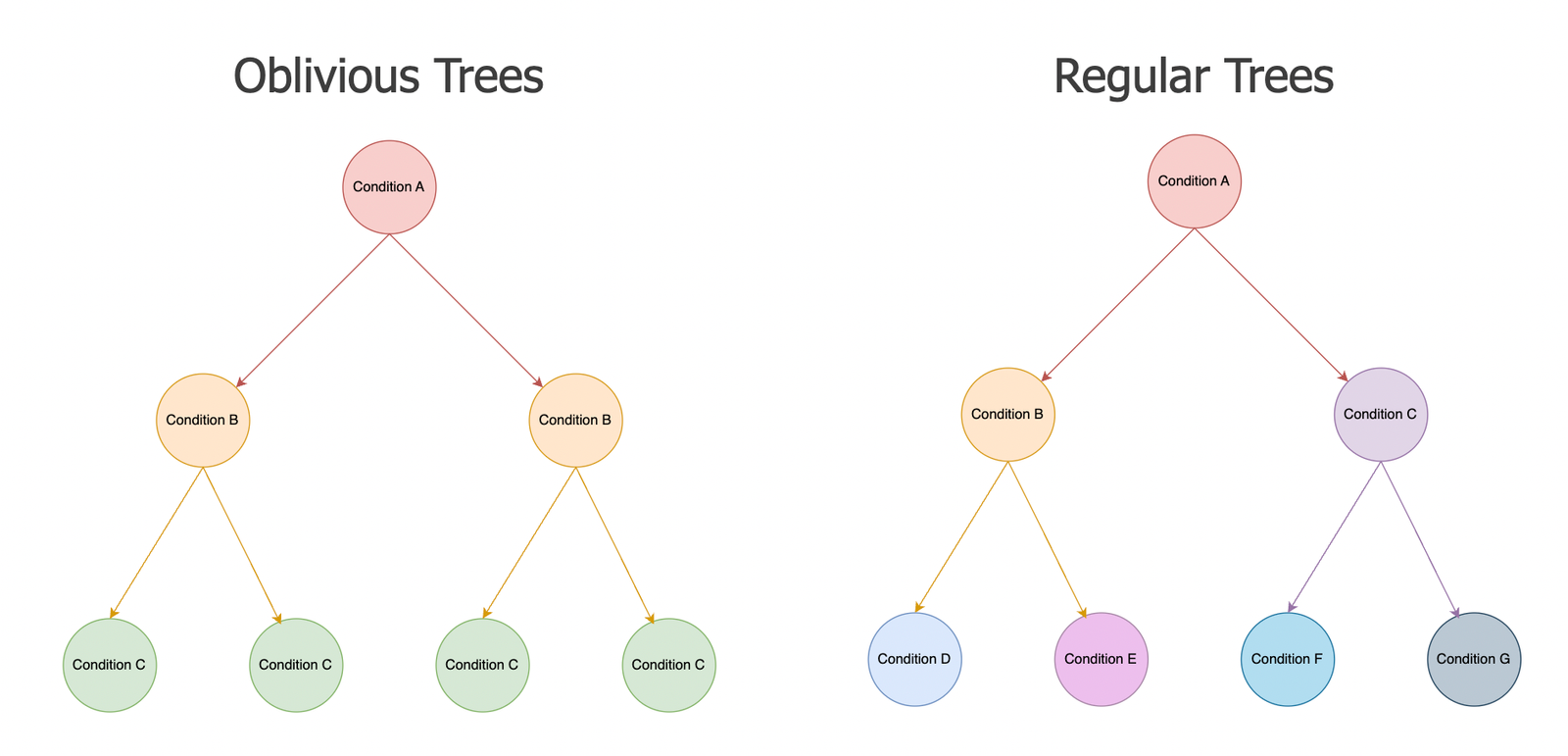
CatBoost makes use of Oblivious Bushes, a key distinction in comparison with different bushes, the place it makes use of the identical cut up throughout all nodes on the identical depth.
Oblivious Bushes

Not like customary determination bushes, the place completely different nodes can cut up on completely different circumstances (feature-threshold), Oblivious Bushes cut up throughout the identical circumstances throughout all nodes on the identical depth of a tree. At a given depth, all samples are evaluated on the identical feature-threshold mixture. This symmetry has a number of implications:
- Velocity and ease: because the identical situation is utilized throughout all nodes on the identical depth, the bushes produced are easier and quicker to coach
- Regularization: Since all bushes are pressured to use the identical situation throughout the tree on the identical depth, there’s a regularization impact on the predictions
- Parallelization: the uniformity of the cut up situation, makes it simpler to parallelize the tree creation and utilization of GPU to speed up coaching
Conclusion
CatBoost stands out by instantly tackling a long-standing problem: tips on how to deal with categorical variables successfully with out inflicting goal leakage. Via improvements like Ordered Goal Statistics, Ordered Boosting, and the usage of Oblivious Bushes, it effectively balances robustness and accuracy.
For those who discovered this deep dive useful, you would possibly get pleasure from one other deep dive on the variations between Stochastic Gradient Classifer and Logistic Regression


