If in case you have carried out a transformer mannequin in PyTorch, you should utilize the identical code for each coaching and inference, however in very other ways. Throughout coaching, you normally course of a batch of fixed-length token sequences and replace the mannequin weights. Throughout inference, the weights are mounted and the mannequin generates new tokens one by one.
This distinction adjustments nearly every part about efficiency. Coaching is dominated by massive matrix multiplications and the backward go. Inference is dominated by repeated ahead passes, reminiscence motion, and the necessity to hold earlier consideration keys and values out there for the following token.
On this chapter, you’ll find out about:
- The autoregressive era loop
- The distinction between prefill and decode
- Why key-value caching is important
- Easy methods to implement a easy KV cache
- Easy methods to cause concerning the reminiscence utilized by the cache
Let’s get began.
Utilizing a Transformer Mannequin: From Coaching to Inference
Photograph by Jacob Smith. Some rights reserved.
Overview
This chapter is split into 4 elements; they’re:
- Autoregressive Technology
- Prefill and Decode
- A Easy KV Cache
- Reminiscence Utilization of the KV Cache
Autoregressive Technology
A decoder-only transformer mannequin predicts the following token from the tokens that got here earlier than it. The strict requirement of utilizing solely the earlier tokens is enforced by the causal consideration mechanism. If the enter tokens are:
the mannequin returns a likelihood distribution over the vocabulary for the following token. A probable subsequent token could also be “mat”, however the mannequin doesn’t return a phrase immediately. It returns logits, that are unnormalized scores for each token within the vocabulary.
The era loop is subsequently easy:
- Tokenize the immediate.
- Run the mannequin to acquire logits for the following token.
- Select a token from the logits.
- Append that token to the enter.
- Repeat till a stopping rule is reached.
That is referred to as autoregressive era as a result of every new token depends upon the earlier generated tokens. The mannequin can’t generate the tenth output token earlier than it is aware of the primary 9 output tokens.
A really small grasping decoding loop could be written as follows:
|
import torch
@torch.no_grad() def greedy_decode(mannequin, input_ids, max_new_tokens): output_ids = input_ids.clone()
for _ in vary(max_new_tokens): logits = mannequin(output_ids) next_token_logits = logits[:, –1, :] next_token = next_token_logits.argmax(dim=–1, keepdim=True) output_ids = torch.cat([output_ids, next_token], dim=1)
return output_ids |
Within the code above, mannequin is a PyTorch mannequin, max_new_tokens is a optimistic integer, and all different variables are PyTorch tensors. The for-loop iterates max_new_tokens occasions, and at every iteration, it feeds your complete sequence again into the mannequin to get the logits for the following token. The argmax() perform selects the highest-scoring token. The cat() perform is used to concatenate the brand new token to the output sequence, which will likely be used within the subsequent iteration till the stopping rule is reached.
This code is simple to grasp, however it’s inefficient. At each iteration, it feeds your complete sequence again into the mannequin. If the immediate has 1,000 tokens and also you generate 100 new tokens, the mannequin repeatedly recomputes the hidden states for a similar immediate tokens. The mannequin processes $O(N^2)$ tokens on this perform, for a immediate of size $N$.
The precise time complexity of the code is even worse. With out caching, each ahead go recomputes consideration for all tokens within the rising sequence. If the sequence size is $N$, self-attention has $O(N^2)$ rating computation. For era, this implies you repeat a considerable amount of work. (Exactly if the output sequence size is $N=P+G$ with immediate size $P$ and variety of generated tokens $G$, the computation complexity ought to be $O(P^2G + PG^2 + G^3)$ naively. With cache, we will cut back it to $O(P^2 + PG)$.)
Inference methods mitigate this by splitting era into two phases: prefill and decode.
Prefill and Decode
Technology normally begins with a immediate. The immediate is thought earlier than era begins. The mannequin can course of all immediate tokens in a single ahead go. That is referred to as the prefill section.
Throughout prefill, the mannequin computes hidden states for all immediate tokens and produces logits for the following token. It additionally computes keys and values for all consideration layers. These keys and values could be saved as a result of they are going to be wanted by each future token.
After the primary new token is chosen, era enters the decode section. In decode, the mannequin receives solely the most recent token. It computes the question, key, and worth for that token, appends the brand new key and worth to the cache, and attends the brand new question over all cached keys and values.
This adjustments the price of one decode step. As an alternative of recomputing consideration for the entire sequence, the mannequin computes consideration for just one new question in opposition to all earlier keys. The per-token consideration value adjustments from roughly $O(N^2)$ to $O(N)$ for a sequence of size $N$. The prefill step continues to be $O(N^2)$, however it’s carried out solely as soon as for the immediate.
This distinction is vital sufficient that serving methods normally measure prefill and decode individually:
- Prefill impacts time to first token. A sluggish prefill will increase time to the primary token.
- Decode impacts the velocity of streaming output tokens. A sluggish decode reduces the speed at which output tokens are streamed.
A brief immediate with an extended reply stresses decode. An extended immediate with a brief reply stresses prefill. A chat software with an extended dialog historical past stresses each.
The matrix under illustrates the attention-score matrix $QK^prime$. Assume the immediate has 5 tokens. Throughout prefill, the mannequin computes the $5 occasions 5$ block in blue. Throughout decode, one new token is added at a time. Every decode step provides one new row to the matrix, proven in a special shade of purple. The weather in black are ignored from calculation because of the causal masks.
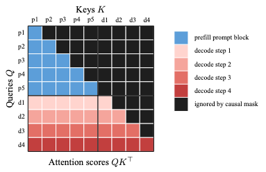
The eye-score matrix grows throughout era. Prefill computes the immediate block as soon as (in blue). Every decode iteration appends one row (as a consequence of expanded $Q$) and one column (as a consequence of expanded $Ok$) for the newly generated token.
A Easy KV Cache
The KV cache is the place the mannequin shops the eye keys and values produced by earlier tokens. To see the way it works, you don’t want a big mannequin. The next code builds a small transformer-like mannequin with a cache.
This mannequin isn’t supposed to provide helpful textual content. Its goal is to point out how the cache is created throughout prefill and prolonged throughout decode.
|
1 2 3 4 5 6 7 8 9 10 11 12 13 14 15 16 17 18 19 20 21 22 23 24 25 26 27 28 29 30 31 32 33 34 35 36 37 38 39 40 41 42 43 44 45 46 47 48 49 50 51 52 53 54 55 56 57 58 59 60 61 62 63 64 65 66 67 68 69 70 71 72 73 74 75 76 77 78 79 80 81 82 83 84 85 86 87 88 89 90 |
import math import torch import torch.nn as nn import torch.nn.practical as F
class SelfAttention(nn.Module): def __init__(self, hidden_size, num_heads): tremendous().__init__() assert hidden_size % num_heads == 0 self.num_heads = num_heads self.head_dim = hidden_size // num_heads self.qkv = nn.Linear(hidden_size, 3 * hidden_size) self.out = nn.Linear(hidden_size, hidden_size)
def ahead(self, x, past_kv=None): # Be aware: Positional encoding and padding masks usually are not carried out right here batch_size, seq_len, hidden_size = x.form
qkv = self.qkv(x) qkv = qkv.view(batch_size, seq_len, 3, self.num_heads, self.head_dim) qkv = qkv.permute(2, 0, 3, 1, 4) q, ok, v = qkv[0], qkv[1], qkv[2]
if past_kv is not None: past_k, past_v = previous_kv ok = torch.cat([past_k, k], dim=2) v = torch.cat([past_v, v], dim=2)
total_len = ok.dimension(2) past_len = total_len – seq_len
scores = q @ ok.transpose(–2, –1) scores = scores / math.sqrt(self.head_dim)
# A token might attend to all cached tokens and earlier tokens # within the present chunk, however not future tokens. causal_mask = torch.ones(seq_len, total_len, machine=x.machine, dtype=torch.bool) causal_mask = torch.tril(causal_mask, diagonal=past_len) scores = scores.masked_fill(~causal_mask, float(“-inf”))
attn = F.softmax(scores, dim=–1) y = attn @ v y = y.transpose(1, 2).contiguous().view(batch_size, seq_len, hidden_size)
return self.out(y), (ok, v)
class Block(nn.Module): def __init__(self, hidden_size, num_heads): tremendous().__init__() self.attn_norm = nn.LayerNorm(hidden_size) self.attn = SelfAttention(hidden_size, num_heads) self.ffn_norm = nn.LayerNorm(hidden_size) self.ffn = nn.Sequential( nn.Linear(hidden_size, 4 * hidden_size), nn.GELU(), nn.Linear(4 * hidden_size, hidden_size), )
def ahead(self, x, past_kv=None): attn_out, new_kv = self.attn(self.attn_norm(x), past_kv=past_kv) x = x + attn_out x = x + self.ffn(self.ffn_norm(x)) return x, new_kv
class TinyCausalLM(nn.Module): def __init__(self, vocab_size=128, hidden_size=64, num_heads=4, num_layers=2): tremendous().__init__() self.token_emb = nn.Embedding(vocab_size, hidden_size) self.blocks = nn.ModuleList([ Block(hidden_size, num_heads) for _ in range(num_layers) ]) self.norm = nn.LayerNorm(hidden_size) self.lm_head = nn.Linear(hidden_size, vocab_size, bias=False)
def ahead(self, input_ids, past_kv=None): x = self.token_emb(input_ids) new_cache = []
if past_kv is None: past_kv = [None] * len(self.blocks)
for block, layer_past in zip(self.blocks, past_kv): x, layer_cache = block(x, past_kv=layer_past) new_cache.append(layer_cache)
logits = self.lm_head(self.norm(x)) return logits, new_cache |
The cache is a listing with one factor per transformer layer. Every factor is a pair (ok, v). The form of every tensor is:
|
[batch_size, num_heads, sequence_length, head_dim] |
Throughout prefill, sequence_length is the immediate size. Throughout decode, the mannequin receives one token at a time and appends one place to the cache.
It’s possible you’ll discover that solely keys and values are saved within the cache however not the question tensor. Be aware that the ahead() methodology is to provide the subsequent token’s logits. To take action, you solely want the final token within the question tensor (which is from the instant earlier token generated) to multiply with each token within the keys to provide consideration scores, that are then used to type a weighted sum of the values. That’s why it’s only a KV cache whereas the eye mechanism is a perform of question, key, and worth.
Here’s a minimal era loop utilizing the cache:
|
1 2 3 4 5 6 7 8 9 10 11 12 13 14 15 16 17 18 19 20 21 22 23 |
torch.no_grad() def greedy_decode_with_cache(mannequin, input_ids, max_new_tokens): output_ids = input_ids.clone()
# Prefill: course of the entire immediate as soon as. logits, cache = mannequin(input_ids) next_token = logits[:, –1, :].argmax(dim=–1, keepdim=True) output_ids = torch.cat([output_ids, next_token], dim=1)
# Decode: course of solely the latest token. assert max_new_tokens > 0, “max_new_tokens should be optimistic” for _ in vary(max_new_tokens – 1): logits, cache = mannequin(next_token, past_kv=cache) next_token = logits[:, –1, :].argmax(dim=–1, keepdim=True) output_ids = torch.cat([output_ids, next_token], dim=1)
return output_ids
mannequin = TinyCausalLM() immediate = torch.tensor([[10, 20, 30, 40]]) generated = greedy_decode_with_cache(mannequin, immediate, max_new_tokens=8) print(generated) |
The mannequin nonetheless produces one token at a time. The distinction is that it not recomputes the immediate tokens after prefill. The important thing logic is in SelfAttention.ahead(): when past_kv is offered, the strategy appends the brand new key and worth to the cached tensors. Throughout decode, the mannequin processes solely essentially the most not too long ago generated next_token somewhat than your complete sequence. That is the essential concept behind the KV cache in manufacturing inference engines.
Reminiscence Utilization of the KV Cache
The KV cache saves compute, but it surely consumes reminiscence. For every token, every layer shops a key tensor and a worth tensor. The approximate reminiscence utilization is:
|
bytes = 2 * num_layers * batch_size * sequence_length * num_kv_heads * head_dim * bytes_per_element |
The issue of 2 is for keys and values. The num_kv_heads worth could also be smaller than the variety of question heads for fashions that use multi-query consideration or grouped-query consideration.
For a mannequin with 32 layers, 32 KV heads, head dimension 128, BF16 cache values, batch dimension 1, and sequence size 4,096:
|
2 * 32 * 1 * 4096 * 32 * 128 * 2 bytes = 2,147,483,648 bytes = 2 GiB |
That is solely the KV cache for one request. It doesn’t embody mannequin weights, non permanent activations, tokenization buffers, or framework overhead. If the service handles many customers concurrently, KV cache reminiscence shortly turns into a limiting issue.
Because of this, an inference system should launch KV cache reminiscence when a request is completed. A easy script can let Python rubbish assortment deal with this, a manufacturing server wants extra environment friendly reminiscence administration, sometimes utilizing cache blocks as a substitute of particular person tensors.
The structure of the cache additionally issues. Within the easy code above, every decode step appends tensors utilizing torch.cat(). That is wonderful for instructing, however it’s inefficient as a result of it repeatedly allocates new tensors and copies previous knowledge. Actual serving engines pre-allocate cache reminiscence prematurely or use a paged structure. Later chapters will revisit this situation intimately.
Environment friendly KV-cache administration is a serious differentiator amongst inference methods.
Additional Studying
Beneath are some sources chances are you’ll discover helpful:
- Consideration Is All You Want, by Vaswani et al.
That is the unique Transformer paper. It introduces scaled dot-product consideration, multi-head consideration, and the query-key-value formulation used all through this chapter. - Consideration (machine studying), on Wikipedia.
This can be a helpful fast reference for the eye mechanism, together with the system $operatorname{softmax}(QK^prime / sqrt{d_k})V$ and the connection between consideration, self-attention, and the Transformer structure. - Quick Transformer Decoding: One Write-Head is All You Want, by Noam Shazeer.
This paper introduces multi-query consideration. It’s immediately associated to inference as a result of it reduces the quantity of key and worth knowledge that should be learn throughout incremental decoding. - FlashAttention: Quick and Reminiscence-Environment friendly Precise Consideration with IO-Consciousness, by Dao et al.
FlashAttention isn’t solely an inference algorithm; the unique paper emphasizes sooner Transformer coaching and memory-efficient actual consideration. It’s nonetheless related to inference as a result of immediate prefill and long-context consideration additionally profit from decreasing reminiscence site visitors and avoiding materializing the total consideration matrix. - Orca: A Distributed Serving System for Transformer-Based mostly Generative Fashions, by Yu et al.
This paper focuses on inference serving. It introduces iteration-level scheduling and selective batching, that are vital concepts behind steady batching for autoregressive era. - Environment friendly Reminiscence Administration for Massive Language Mannequin Serving with PagedAttention, by Kwon et al.
This paper is immediately about LLM inference serving. PagedAttention shops the KV cache in fixed-size blocks as a substitute of requiring every request’s cache to be contiguous, decreasing reminiscence fragmentation and permitting bigger batches.
Abstract
On this article, you discovered that inference is not only coaching with out the backward go. The mannequin is utilized in a special sample: one prefill step adopted by many decode steps. The KV cache avoids recomputing consideration keys and values for earlier tokens, altering the per-token consideration value throughout decode from quadratic to linear within the sequence size.
You additionally carried out a easy KV cache in a tiny transformer mannequin. This cache is the inspiration for a lot of later optimizations, together with paged consideration, steady batching, prefix caching, long-context inference, and disaggregated prefill and decode.
If in case you have carried out a transformer mannequin in PyTorch, you should utilize the identical code for each coaching and inference, however in very other ways. Throughout coaching, you normally course of a batch of fixed-length token sequences and replace the mannequin weights. Throughout inference, the weights are mounted and the mannequin generates new tokens one by one.
This distinction adjustments nearly every part about efficiency. Coaching is dominated by massive matrix multiplications and the backward go. Inference is dominated by repeated ahead passes, reminiscence motion, and the necessity to hold earlier consideration keys and values out there for the following token.
On this chapter, you’ll find out about:
- The autoregressive era loop
- The distinction between prefill and decode
- Why key-value caching is important
- Easy methods to implement a easy KV cache
- Easy methods to cause concerning the reminiscence utilized by the cache
Let’s get began.
Utilizing a Transformer Mannequin: From Coaching to Inference
Photograph by Jacob Smith. Some rights reserved.
Overview
This chapter is split into 4 elements; they’re:
- Autoregressive Technology
- Prefill and Decode
- A Easy KV Cache
- Reminiscence Utilization of the KV Cache
Autoregressive Technology
A decoder-only transformer mannequin predicts the following token from the tokens that got here earlier than it. The strict requirement of utilizing solely the earlier tokens is enforced by the causal consideration mechanism. If the enter tokens are:
the mannequin returns a likelihood distribution over the vocabulary for the following token. A probable subsequent token could also be “mat”, however the mannequin doesn’t return a phrase immediately. It returns logits, that are unnormalized scores for each token within the vocabulary.
The era loop is subsequently easy:
- Tokenize the immediate.
- Run the mannequin to acquire logits for the following token.
- Select a token from the logits.
- Append that token to the enter.
- Repeat till a stopping rule is reached.
That is referred to as autoregressive era as a result of every new token depends upon the earlier generated tokens. The mannequin can’t generate the tenth output token earlier than it is aware of the primary 9 output tokens.
A really small grasping decoding loop could be written as follows:
|
import torch
@torch.no_grad() def greedy_decode(mannequin, input_ids, max_new_tokens): output_ids = input_ids.clone()
for _ in vary(max_new_tokens): logits = mannequin(output_ids) next_token_logits = logits[:, –1, :] next_token = next_token_logits.argmax(dim=–1, keepdim=True) output_ids = torch.cat([output_ids, next_token], dim=1)
return output_ids |
Within the code above, mannequin is a PyTorch mannequin, max_new_tokens is a optimistic integer, and all different variables are PyTorch tensors. The for-loop iterates max_new_tokens occasions, and at every iteration, it feeds your complete sequence again into the mannequin to get the logits for the following token. The argmax() perform selects the highest-scoring token. The cat() perform is used to concatenate the brand new token to the output sequence, which will likely be used within the subsequent iteration till the stopping rule is reached.
This code is simple to grasp, however it’s inefficient. At each iteration, it feeds your complete sequence again into the mannequin. If the immediate has 1,000 tokens and also you generate 100 new tokens, the mannequin repeatedly recomputes the hidden states for a similar immediate tokens. The mannequin processes $O(N^2)$ tokens on this perform, for a immediate of size $N$.
The precise time complexity of the code is even worse. With out caching, each ahead go recomputes consideration for all tokens within the rising sequence. If the sequence size is $N$, self-attention has $O(N^2)$ rating computation. For era, this implies you repeat a considerable amount of work. (Exactly if the output sequence size is $N=P+G$ with immediate size $P$ and variety of generated tokens $G$, the computation complexity ought to be $O(P^2G + PG^2 + G^3)$ naively. With cache, we will cut back it to $O(P^2 + PG)$.)
Inference methods mitigate this by splitting era into two phases: prefill and decode.
Prefill and Decode
Technology normally begins with a immediate. The immediate is thought earlier than era begins. The mannequin can course of all immediate tokens in a single ahead go. That is referred to as the prefill section.
Throughout prefill, the mannequin computes hidden states for all immediate tokens and produces logits for the following token. It additionally computes keys and values for all consideration layers. These keys and values could be saved as a result of they are going to be wanted by each future token.
After the primary new token is chosen, era enters the decode section. In decode, the mannequin receives solely the most recent token. It computes the question, key, and worth for that token, appends the brand new key and worth to the cache, and attends the brand new question over all cached keys and values.
This adjustments the price of one decode step. As an alternative of recomputing consideration for the entire sequence, the mannequin computes consideration for just one new question in opposition to all earlier keys. The per-token consideration value adjustments from roughly $O(N^2)$ to $O(N)$ for a sequence of size $N$. The prefill step continues to be $O(N^2)$, however it’s carried out solely as soon as for the immediate.
This distinction is vital sufficient that serving methods normally measure prefill and decode individually:
- Prefill impacts time to first token. A sluggish prefill will increase time to the primary token.
- Decode impacts the velocity of streaming output tokens. A sluggish decode reduces the speed at which output tokens are streamed.
A brief immediate with an extended reply stresses decode. An extended immediate with a brief reply stresses prefill. A chat software with an extended dialog historical past stresses each.
The matrix under illustrates the attention-score matrix $QK^prime$. Assume the immediate has 5 tokens. Throughout prefill, the mannequin computes the $5 occasions 5$ block in blue. Throughout decode, one new token is added at a time. Every decode step provides one new row to the matrix, proven in a special shade of purple. The weather in black are ignored from calculation because of the causal masks.
The eye-score matrix grows throughout era. Prefill computes the immediate block as soon as (in blue). Every decode iteration appends one row (as a consequence of expanded $Q$) and one column (as a consequence of expanded $Ok$) for the newly generated token.
A Easy KV Cache
The KV cache is the place the mannequin shops the eye keys and values produced by earlier tokens. To see the way it works, you don’t want a big mannequin. The next code builds a small transformer-like mannequin with a cache.
This mannequin isn’t supposed to provide helpful textual content. Its goal is to point out how the cache is created throughout prefill and prolonged throughout decode.
|
1 2 3 4 5 6 7 8 9 10 11 12 13 14 15 16 17 18 19 20 21 22 23 24 25 26 27 28 29 30 31 32 33 34 35 36 37 38 39 40 41 42 43 44 45 46 47 48 49 50 51 52 53 54 55 56 57 58 59 60 61 62 63 64 65 66 67 68 69 70 71 72 73 74 75 76 77 78 79 80 81 82 83 84 85 86 87 88 89 90 |
import math import torch import torch.nn as nn import torch.nn.practical as F
class SelfAttention(nn.Module): def __init__(self, hidden_size, num_heads): tremendous().__init__() assert hidden_size % num_heads == 0 self.num_heads = num_heads self.head_dim = hidden_size // num_heads self.qkv = nn.Linear(hidden_size, 3 * hidden_size) self.out = nn.Linear(hidden_size, hidden_size)
def ahead(self, x, past_kv=None): # Be aware: Positional encoding and padding masks usually are not carried out right here batch_size, seq_len, hidden_size = x.form
qkv = self.qkv(x) qkv = qkv.view(batch_size, seq_len, 3, self.num_heads, self.head_dim) qkv = qkv.permute(2, 0, 3, 1, 4) q, ok, v = qkv[0], qkv[1], qkv[2]
if past_kv is not None: past_k, past_v = previous_kv ok = torch.cat([past_k, k], dim=2) v = torch.cat([past_v, v], dim=2)
total_len = ok.dimension(2) past_len = total_len – seq_len
scores = q @ ok.transpose(–2, –1) scores = scores / math.sqrt(self.head_dim)
# A token might attend to all cached tokens and earlier tokens # within the present chunk, however not future tokens. causal_mask = torch.ones(seq_len, total_len, machine=x.machine, dtype=torch.bool) causal_mask = torch.tril(causal_mask, diagonal=past_len) scores = scores.masked_fill(~causal_mask, float(“-inf”))
attn = F.softmax(scores, dim=–1) y = attn @ v y = y.transpose(1, 2).contiguous().view(batch_size, seq_len, hidden_size)
return self.out(y), (ok, v)
class Block(nn.Module): def __init__(self, hidden_size, num_heads): tremendous().__init__() self.attn_norm = nn.LayerNorm(hidden_size) self.attn = SelfAttention(hidden_size, num_heads) self.ffn_norm = nn.LayerNorm(hidden_size) self.ffn = nn.Sequential( nn.Linear(hidden_size, 4 * hidden_size), nn.GELU(), nn.Linear(4 * hidden_size, hidden_size), )
def ahead(self, x, past_kv=None): attn_out, new_kv = self.attn(self.attn_norm(x), past_kv=past_kv) x = x + attn_out x = x + self.ffn(self.ffn_norm(x)) return x, new_kv
class TinyCausalLM(nn.Module): def __init__(self, vocab_size=128, hidden_size=64, num_heads=4, num_layers=2): tremendous().__init__() self.token_emb = nn.Embedding(vocab_size, hidden_size) self.blocks = nn.ModuleList([ Block(hidden_size, num_heads) for _ in range(num_layers) ]) self.norm = nn.LayerNorm(hidden_size) self.lm_head = nn.Linear(hidden_size, vocab_size, bias=False)
def ahead(self, input_ids, past_kv=None): x = self.token_emb(input_ids) new_cache = []
if past_kv is None: past_kv = [None] * len(self.blocks)
for block, layer_past in zip(self.blocks, past_kv): x, layer_cache = block(x, past_kv=layer_past) new_cache.append(layer_cache)
logits = self.lm_head(self.norm(x)) return logits, new_cache |
The cache is a listing with one factor per transformer layer. Every factor is a pair (ok, v). The form of every tensor is:
|
[batch_size, num_heads, sequence_length, head_dim] |
Throughout prefill, sequence_length is the immediate size. Throughout decode, the mannequin receives one token at a time and appends one place to the cache.
It’s possible you’ll discover that solely keys and values are saved within the cache however not the question tensor. Be aware that the ahead() methodology is to provide the subsequent token’s logits. To take action, you solely want the final token within the question tensor (which is from the instant earlier token generated) to multiply with each token within the keys to provide consideration scores, that are then used to type a weighted sum of the values. That’s why it’s only a KV cache whereas the eye mechanism is a perform of question, key, and worth.
Here’s a minimal era loop utilizing the cache:
|
1 2 3 4 5 6 7 8 9 10 11 12 13 14 15 16 17 18 19 20 21 22 23 |
torch.no_grad() def greedy_decode_with_cache(mannequin, input_ids, max_new_tokens): output_ids = input_ids.clone()
# Prefill: course of the entire immediate as soon as. logits, cache = mannequin(input_ids) next_token = logits[:, –1, :].argmax(dim=–1, keepdim=True) output_ids = torch.cat([output_ids, next_token], dim=1)
# Decode: course of solely the latest token. assert max_new_tokens > 0, “max_new_tokens should be optimistic” for _ in vary(max_new_tokens – 1): logits, cache = mannequin(next_token, past_kv=cache) next_token = logits[:, –1, :].argmax(dim=–1, keepdim=True) output_ids = torch.cat([output_ids, next_token], dim=1)
return output_ids
mannequin = TinyCausalLM() immediate = torch.tensor([[10, 20, 30, 40]]) generated = greedy_decode_with_cache(mannequin, immediate, max_new_tokens=8) print(generated) |
The mannequin nonetheless produces one token at a time. The distinction is that it not recomputes the immediate tokens after prefill. The important thing logic is in SelfAttention.ahead(): when past_kv is offered, the strategy appends the brand new key and worth to the cached tensors. Throughout decode, the mannequin processes solely essentially the most not too long ago generated next_token somewhat than your complete sequence. That is the essential concept behind the KV cache in manufacturing inference engines.
Reminiscence Utilization of the KV Cache
The KV cache saves compute, but it surely consumes reminiscence. For every token, every layer shops a key tensor and a worth tensor. The approximate reminiscence utilization is:
|
bytes = 2 * num_layers * batch_size * sequence_length * num_kv_heads * head_dim * bytes_per_element |
The issue of 2 is for keys and values. The num_kv_heads worth could also be smaller than the variety of question heads for fashions that use multi-query consideration or grouped-query consideration.
For a mannequin with 32 layers, 32 KV heads, head dimension 128, BF16 cache values, batch dimension 1, and sequence size 4,096:
|
2 * 32 * 1 * 4096 * 32 * 128 * 2 bytes = 2,147,483,648 bytes = 2 GiB |
That is solely the KV cache for one request. It doesn’t embody mannequin weights, non permanent activations, tokenization buffers, or framework overhead. If the service handles many customers concurrently, KV cache reminiscence shortly turns into a limiting issue.
Because of this, an inference system should launch KV cache reminiscence when a request is completed. A easy script can let Python rubbish assortment deal with this, a manufacturing server wants extra environment friendly reminiscence administration, sometimes utilizing cache blocks as a substitute of particular person tensors.
The structure of the cache additionally issues. Within the easy code above, every decode step appends tensors utilizing torch.cat(). That is wonderful for instructing, however it’s inefficient as a result of it repeatedly allocates new tensors and copies previous knowledge. Actual serving engines pre-allocate cache reminiscence prematurely or use a paged structure. Later chapters will revisit this situation intimately.
Environment friendly KV-cache administration is a serious differentiator amongst inference methods.
Additional Studying
Beneath are some sources chances are you’ll discover helpful:
- Consideration Is All You Want, by Vaswani et al.
That is the unique Transformer paper. It introduces scaled dot-product consideration, multi-head consideration, and the query-key-value formulation used all through this chapter. - Consideration (machine studying), on Wikipedia.
This can be a helpful fast reference for the eye mechanism, together with the system $operatorname{softmax}(QK^prime / sqrt{d_k})V$ and the connection between consideration, self-attention, and the Transformer structure. - Quick Transformer Decoding: One Write-Head is All You Want, by Noam Shazeer.
This paper introduces multi-query consideration. It’s immediately associated to inference as a result of it reduces the quantity of key and worth knowledge that should be learn throughout incremental decoding. - FlashAttention: Quick and Reminiscence-Environment friendly Precise Consideration with IO-Consciousness, by Dao et al.
FlashAttention isn’t solely an inference algorithm; the unique paper emphasizes sooner Transformer coaching and memory-efficient actual consideration. It’s nonetheless related to inference as a result of immediate prefill and long-context consideration additionally profit from decreasing reminiscence site visitors and avoiding materializing the total consideration matrix. - Orca: A Distributed Serving System for Transformer-Based mostly Generative Fashions, by Yu et al.
This paper focuses on inference serving. It introduces iteration-level scheduling and selective batching, that are vital concepts behind steady batching for autoregressive era. - Environment friendly Reminiscence Administration for Massive Language Mannequin Serving with PagedAttention, by Kwon et al.
This paper is immediately about LLM inference serving. PagedAttention shops the KV cache in fixed-size blocks as a substitute of requiring every request’s cache to be contiguous, decreasing reminiscence fragmentation and permitting bigger batches.
Abstract
On this article, you discovered that inference is not only coaching with out the backward go. The mannequin is utilized in a special sample: one prefill step adopted by many decode steps. The KV cache avoids recomputing consideration keys and values for earlier tokens, altering the per-token consideration value throughout decode from quadratic to linear within the sequence size.
You additionally carried out a easy KV cache in a tiny transformer mannequin. This cache is the inspiration for a lot of later optimizations, together with paged consideration, steady batching, prefix caching, long-context inference, and disaggregated prefill and decode.