The Machine Studying “Creation Calendar” Day 4: k-Means in Excel

Through the first three days, we explored distance-based fashions for supervised studying:

In all these fashions, the thought was the identical: we measure distances, and we resolve the output primarily based on the closest factors or nearest facilities.

At the moment, we keep on this similar household of concepts. However we use the distances in an unsupervised method: k-means.

Now, one query for many who already know this algorithm: k-means seems extra much like which mannequin, the k-NN classifier, or the Nearest Centroid classifier?

And should you bear in mind, for all of the fashions we have now seen to this point, there was probably not a “coaching” part or hyperparameter tuning.

For k-NN, there isn’t any coaching in any respect.

For LDA, QDA, or GNB, coaching is simply computing means and variances. And there are additionally no actual hyperparameters.

Now, with k-means, we’re going to implement a coaching algorithm that lastly seems like “actual” machine studying.

We begin with a tiny 1D instance. Then we transfer to 2D.

Purpose of k-means

Within the coaching dataset, there are no preliminary labels.

The aim of k-means is to create significant labels by grouping factors which are shut to one another.

Allow us to take a look at the illustration under. You may clearly see two teams of factors. Every centroid (the pink sq. and the inexperienced sq.) is in the midst of its cluster, and each level is assigned to the closest one.

This provides a really intuitive image of how k-means discovers construction utilizing solely distances.

And right here, okay means the variety of facilities we attempt to discover.

Now, allow us to reply the query: Which algorithm is k-means nearer to, the k-NN classifier or the Nearest Centroid classifier?

Don’t be fooled by the okay in k-NN and k-means.
They don’t imply the identical factor:

in k-NN, okay is the variety of neighbors, not the variety of lessons;
in k-means, okay is the variety of centroids.

Ok-means is way nearer to the Nearest Centroid classifier.

Each fashions are represented by centroids, and for a brand new commentary we merely compute the gap to every centroid to resolve to which one it belongs.

The distinction, in fact, is that within the Nearest Centroid classifier, we already know the centroids as a result of they arrive from labeled lessons.

In k-means, we have no idea the centroids. The entire aim of the algorithm is to uncover appropriate ones immediately from the information.

The enterprise drawback is totally completely different: as a substitute of predicting labels, we are attempting to create them.

And in k-means, the worth of okay (the variety of centroids) is unknown. So it turns into a hyperparameter that we will tune.

k-means with solely One characteristic

We begin with a tiny 1D instance in order that the whole lot is seen on one axis. And we are going to select the values in such a trivial method that we will immediately see the 2 centroids.

1, 2, 3, 11, 12, 13

Sure, 2, and 12.

However how would the pc know? The machine will “be taught” by guessing step-by-step.

Right here comes the algorithm known as Lloyd’s algorithm.

We are going to implement it in Excel with the next loop:

select preliminary centroids
compute the gap from every level to every centroid
assign every level to the closest centroid
recompute the centroids as the common of the factors in every cluster
repeat steps 2 to 4 till the centroids not transfer

1. Select preliminary centroids

Choose two preliminary facilities, for instance:

They need to be inside the information vary (between 1 and 13).

2. Compute distances

For every information level x:

compute the gap to c_1,
compute the gap to c_2.

Sometimes, we use absolute distance in 1D.

We now have two distance values for every level.

3. Assign clusters

For every level:

examine the 2 distances,
assign the cluster of the smallest one (1 or 2).

In Excel, this can be a easy IF or MIN primarily based logic.

4. Compute the brand new centroids

For every cluster:

take the factors assigned to that cluster,
compute their common,
this common turns into the brand new centroid.

5. Iterate till reaching convergence

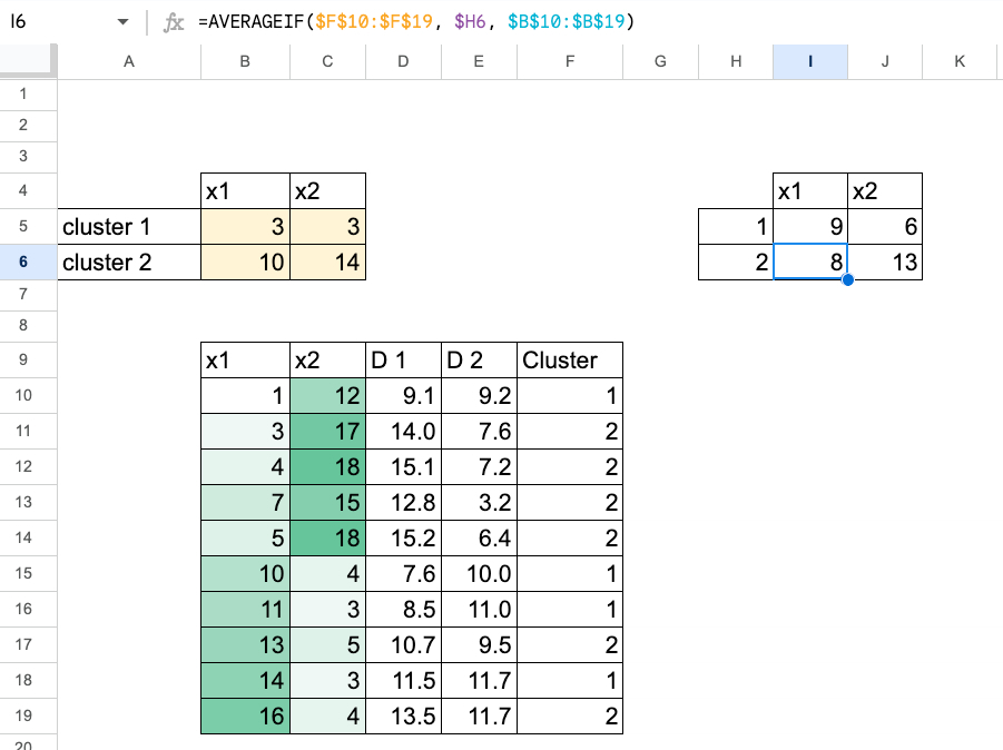
Now in Excel, due to the formulation, we will merely paste the brand new centroid values into the cells of the preliminary centroids.

The replace is instant, and after doing this a couple of occasions, you will note that the values cease altering. That’s when the algorithm has converged.

We are able to additionally document every step in Excel, so we will see how the centroids and clusters evolve over time.

k-means with Two Options

Now allow us to use two options. The method is strictly the identical, we merely use the Euclidean distance in 2D.

You may both do the copy-paste of the brand new centroids as values (with only a few cells to replace),

or you possibly can show all of the intermediate steps to see the complete evolution of the algorithm.

Visualizing the Shifting Centroids in Excel

To make the method extra intuitive, it’s useful to create plots that present how the centroids transfer.

Sadly, Excel or Google Sheets should not ideally suited for this sort of visualization, and the information tables shortly change into a bit advanced to arrange.

If you wish to see a full instance with detailed plots, you possibly can learn this text I wrote nearly three years in the past, the place every step of the centroid motion is proven clearly.

As you possibly can see on this image, the worksheet turned fairly unorganized, particularly in comparison with the sooner desk, which was very simple.

Selecting the optimum okay: The Elbow Methodology

So now, it’s attainable to strive okay = 2 and okay = 3 in our case, and compute the inertia for every one. Then we merely examine the values.

We are able to even start with okay=1.

For every worth of okay:

we run k-Means till convergence,
compute the inertia, which is the sum of squared distances between every level and its assigned centroid.

In Excel:

For every level, take the gap to its centroid and sq. it.
Sum all these squared distances.
This provides the inertia for this okay.

For instance:

for okay = 1, the centroid is simply the general imply of x1 and x2,
for okay = 2 and okay = 3, we take the converged centroids from the sheets the place you ran the algorithm.

Then we will plot inertia as a operate of okay, for instance for (okay = 1, 2, 3).

For this dataset

from 1 to 2, the inertia drops so much,
from 2 to three, the advance is way smaller.

The “elbow” is the worth of okay after which the lower in inertia turns into marginal. Within the instance, it means that okay = 2 is ample.

Conclusion

Ok-means is a really intuitive algorithm when you see it step-by-step in Excel.

We begin with easy centroids, compute distances, assign factors, replace the centroids, and repeat. Now, we will see how “machines be taught”, proper?

Nicely, that is solely the start, we are going to see that completely different fashions “be taught” in actually alternative ways.

And right here is the transition for tomorrow’s article: the unsupervised model of the Nearest Centroid classifier is certainly k-means.

So what can be the unsupervised model of LDA or QDA? We are going to reply this within the subsequent article.