


any time with Transformers, you already know consideration is the mind of the entire operation. It’s what lets the mannequin work out which tokens are speaking to one another, and that one mechanism is chargeable for nearly all the pieces spectacular LLMs do.
Consideration works with three elements: Question (Q), Key (Okay), and Worth (V) [1]. The dot product between Q and Okay is what tells the mannequin how a lot every token ought to give attention to the others, and that’s basically the core of what consideration does.
Now, calling consideration the “mind” additionally means it comes with a price. Throughout inference, each time a brand new token is being predicted, the Okay and V matrices are recalculated for all of the earlier tokens too. So if 90 tokens are already there and the mannequin is predicting the 91st, it goes again and recomputes KV for all 90. Isn’t this repetitiveness a waste?
KV cache modified this. The thought is easy, as a substitute of recomputing, simply retailer the Okay and V matrices in VRAM and reuse them throughout inference. Sounds easy, proper? Which might be why each main LLM on the market has adopted it, the drop in latency is difficult to argue with.
Although KV cache got here as a silver lining for LLMs, it introduced up extra challenges. It launched further reminiscence overhead. This may not be an enormous problem for SLMs, however mega-LLMs with billions of parameters now grew to become tougher to load on machines. Roughly 20-30% further VRAM is consumed by the KV cache alone. The larger limitation is that this overhead isn’t static, it retains rising. This could develop as much as the mannequin dimension itself with lengthy contexts or extra concurrent customers, since every consumer will get their very own KV cache. To resolve this many researchers launched completely different approaches like Grouped-Question Consideration (GQA) [2], PagedAttention (VLLM) [3], Quantization (to 4-bit or 8-bit). Nonetheless, all of those helped with the reminiscence overhead problem however accuracy needed to be compromised for that. There was no resolution to each compress them and retain authentic accuracy. Then got here TurboQuant from Google, which surprisingly manages to do each. The authors additionally show that this resolution sits on the theoretical optimum, the very best for this class of drawback.
TurboQuant comes with two phases: PolarQuant and Residual Correction [4].
PolarQuant (Stage 1): Compresses the Okay and V matrices.
Residual Correction (Stage 2): Corrects the quantization error left after PolarQuant, recovering misplaced info.
Making use of each sequentially is what makes it completely different from conventional quantization. Here’s a visible breakdown:

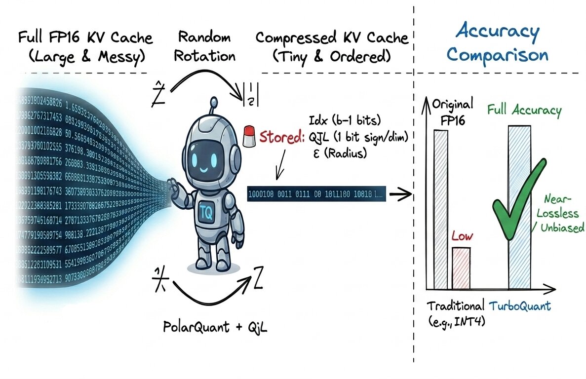
That ought to offer you a transparent image of the pipeline of TurboQuant and the way it differs from the standard quantization we talked about. Earlier than we dive into every stage, allow us to uncover one other essential factor: since we’re speaking about lowering the reminiscence overhead, what precisely does TurboQuant retailer in cache? and the way a lot much less reminiscence does it really take up? Allow us to look into that visually beneath:

You may not totally grasp what Idx, QJL, and ε imply simply but, however they’ll develop into clear as we unpack this pipeline step-by-step. For now, the desk above offers you the important concept: it exhibits precisely what TurboQuant shops in contrast with conventional quantization.
The important thing takeaway? Though each methods obtain equivalent compression charges (the additional ε scalar is negligible when you unfold it throughout the vector dimensions), TurboQuant retains accuracy on par with the unique full-precision mannequin. In actual fact, the official paper reviews that TurboQuant delivers greater than 4.5–5x KV cache compression, that’s efficient 3.5–2.5 bits per channel, with near-zero accuracy loss in apply. That’s fairly phenomenal.
Now let’s stroll by means of the precise step-by-step move of TurboQuant, the precise sequence we previewed within the diagram earlier.
Stage 1 (PolarQuant):
This entails two main operations in it, Rotation and LLoyd Max Quantization.
However why rotation within the first place? The foremost flaw of conventional quantization is how badly it handles outliers. To make this concrete, lets assume we have now a 4 dimensional key vector for a token: [0.125, 0.103, 0.220, 6.030] (Outliers like this are literally fairly widespread in consideration keys). Now if we quantize them historically, the quantizer has to stretch its restricted ranges to cowl that huge 6.030 spike. The consequence? One thing like [0, 0, 0, 1], nearly all the data is misplaced.
Rotating the vector resolves this problem. This “spinning” of vector in high-dimensional area (y = R*x, the place R is random orthogonal rotation matrix) removes the spike and immerses its vitality to the opposite coordinates making the vector distribution easy (Isotropic). The values are modified however the total magnitude stays the identical. After rotation, the identical instance vector would possibly look one thing extra balanced like [1.42, -0.85, 2.31, 0.97].

This smoothed distribution for high-dimensional vectors brings us near gaussian distribution (in apply, the rotated vector is uniformly distributed on the unit sphere, as anticipated from the central restrict theorem). Consequently, every coordinate thus follows beta-like distribution over the vitality current within the vector.
the place d is head dimension
Tip (skip when you’re not into the maths particulars): That is linked to a basic property in multivariate statistics, the place if X1, X2, …. Xd ~ N(0,1) are impartial and identically distributed (i.i.d), then Xi2 ~ Chi-Squared distribution and there’s a theorem which states that:
Now rotation has led us to the purpose that we all know what’s the distribution like of coordinates. Now comes second main operation in stage 1: Lloyd Max Quantization:
The entire concept behind Lloyd-Max [5,6] is to position the quantization ranges (centroids) in precisely the proper spots so the imply squared error is minimized. It’s principally good clustering for 1D knowledge. Let’s simplify it with an instance. Taking the identical rotated vector as above: [1.42, -0.85, 2.31, 0.97]. Suppose we’re doing 1 bit quantization right here.
- Variety of centroids or ranges listed here are 2bits = 21 = 2.
- Allow us to take preliminary random ranges as [0.5, 1.5], their mid-point or boundary is (0.5 + 1.5)/2 ~ 1, thus the quantized values now develop into [1.5, 0.5, 1.5, 0.5] (All values beneath 1 belong to 0.5 and above 1 belong to 1.5). That’s the concept of quantization proper? however what we discover is there’s a lot of error right here, i.e., MSE could be very excessive.
- Thus we have now to seek out optimum ranges such that MSE is minimal and values are finest represented round them.
- That is achieved by Llyod Max quantization: since now new values are [1.5, 0.5, 1.5, 0.5], allotting two clusters:
-0.85, 0.97 –> 0.5 degree cluster,
1.42, 2.31 –> 1.5 degree cluster.
Taking their imply, 0.5 degree cluster imply ~ 0.06 and 1.5 cluster imply ~ 1.86.
So now the brand new ranges are modified from [0.5, 1.5] to [0.06, 1.86], and our new boundary now could be (0.06+1.86)/2 ~ 0.96, now values decrease than 0.96 belong to 0.06 degree and values above 0.96 belong to 1.86. This retains on reiterating till we attain a degree the place MSE doesn’t enhance.
Tip: There’s a basic statistical cause this works: the worth that minimizes squared error for any group of factors is solely their imply.
However wait, operating this repetitive course of on each new vector throughout inference can be manner too gradual, proper? Right here’s the place the rotation pays off once more. As a result of each coordinate now follows the identical recognized distribution (the Beta we noticed earlier), we don’t need to compute a recent Lloyd-Max codebook for each new piece of information. As an alternative, the optimum codebook relies upon solely on two fastened parameters: the head dimension (d) and the variety of bits (b). We compute it as soon as, offline, and reuse it ceaselessly. A snippet of this codebook is proven beneath:

The quantized values usually are not saved in float, however within the type of indexes (idx) of ranges. Instance: if the degrees have been 8, then its listed (idx) kind is 0, 1, 2, 3, 4, 5, 6, 7. Thus needing 3 bits for storage of every worth.
Word: In TurboQuant’s Stage 1 (PolarQuant), the precise saved index (idx) makes use of b-1 bits per dimension (codebook dimension = 2{b-1}), not b bits. The additional bit per dimension comes from the QJL residual correction in Stage 2 (Similar was talked about in storage comparability diagram of this text above, hope now it’s clear) The desk above exhibits the final Lloyd-Max setup; TurboQuant cleverly splits the finances to go away room for that correction.
These indexes are saved in cache till the token is evicted. Dequantization occurs on the fly at any time when that token’s Okay is required for consideration, idx is appeared up within the codebook to retrieve the float values for every index, and this matrix is then multiplied with the transpose of the unique rotation matrix to get again Okaŷ within the authentic area. This completes the primary stage.
Due to this fact, lastly we’re capable of extract residuals:
ε = Authentic Okay matrix – Okaŷ matrix [dequantized]
Stage 2 (Residual Correction):
Now that we have now the residuals, essentially the most intriguing a part of TurboQuant follows.
Conventional quantization didn’t even look into the residuals. Nonetheless TurboQuant doesn’t discard this residual. As an alternative it asks a intelligent query, no matter info was misplaced throughout Stage 1 compression, can we extract its important traits moderately than storing it totally? Consider it as asking easy sure/no questions in regards to the residual: is that this dimension leaning constructive or adverse? The solutions to those sure/no questions are what Stage 2 preserves.
To do that, a random projection matrix S of form (d, d) is multiplied with the residual vector. The indicators of the ensuing values, both +1 or -1, are what really get saved.
Signal(ε(seq_length, d) * S(d, d))
These signal projections are referred to as the Quantized Johnson-Lindenstrauss (QJL) Remodel [7].
Word: The randomness of S isn’t arbitrary, the Johnson-Lindenstrauss lemma ensures that random projections protect internal product construction with excessive likelihood.
However indicators alone solely seize path, not magnitude. So alongside QJL, the L2 norm of the residual (‖ε‖₂) can also be saved as a single scalar per vector. This scalar is what restores the magnitude throughout reconstruction.
Throughout dequantization, these saved signal bits are multiplied again with transposed S, then scaled by (√π/2)/d and the saved norm ‖ε‖₂. The authors present that with out this scaling issue, the sign-based estimation of the internal product is biased, this correction is what makes it unbiased. The precise components is proven beneath:
Lastly the 2 components from each phases are added collectively to get:
Okaỹ = Okaŷ + OkaỹQJL
A number of the final minute observations:
- Full TurboQuant pipeline summed up: Stage 1 handles the majority compression, Stage 2 hunts down what was misplaced and provides it again.
- So what really sits in cache for every token is three issues: Idx, the signal bits QJL, and the scalar norm ‖ε‖₂. That’s the full compressed illustration.
- The authors formally show that this two-stage design reaches the theoretical optimum, which means no technique working throughout the identical bit finances can do higher at preserving consideration dot merchandise.
Conclusion:
On the finish of the day, TurboQuant works as a result of it stops obsessing over good vector reconstruction and cleverly focuses on what the eye mechanism really must see. As an alternative of combating the VRAM “tax” with extra advanced calibration, it simply makes use of a cleaner mathematical pipeline to get the job achieved.
As we hold pushing for longer context home windows, the KV cache bottleneck isn’t going away. However as this framework exhibits, we don’t essentially want extra {hardware}, we simply should be extra intentional about how we deal with the info we have already got.
With the introduction of TurboQuant, is the chapter of KV Cache reminiscence administration lastly closed? Or is that this simply the inspiration for one thing much more highly effective?
Word: This breakdown represents my present understanding of the TurboQuant pipeline. Any errors in interpretation are totally my very own, and I encourage readers to confer with the unique analysis for the total mathematical proofs.
References:
[1] Vaswani, A., et al. (2017). Consideration Is All You Want. Advances in Neural Info Processing Techniques (NeurIPS 2017).
[2] Ainslie, J., et al. (2023). GQA: Coaching Generalized Multi-Question Transformer Fashions from Multi-Head Checkpoints. EMNLP 2023.
[3] Kwon, W., et al. (2023). Environment friendly Reminiscence Administration for Massive Language Mannequin Serving with PagedAttention. SOSP 2023.
[4] Zandieh, A., et al. (2025). TurboQuant: On-line Vector Quantization with Close to-optimal Distortion Fee. arXiv:2504.19874.
[5] Lloyd, S. P. (1982). Least Squares Quantization in PCM. IEEE Transactions on Info Principle, 28(2), 129–137.
[6] Max, J. (1960). Quantizing for Minimal Distortion. IRE Transactions on Info Principle, 6(1), 7–12.
[7] Zandieh, A., et al. (2024). QJL: 1-Bit Quantized JL Remodel for KV Cache Quantization with Zero Overhead. AAAI 2025.


