Exploring Patterns of Survival from the Titanic Dataset

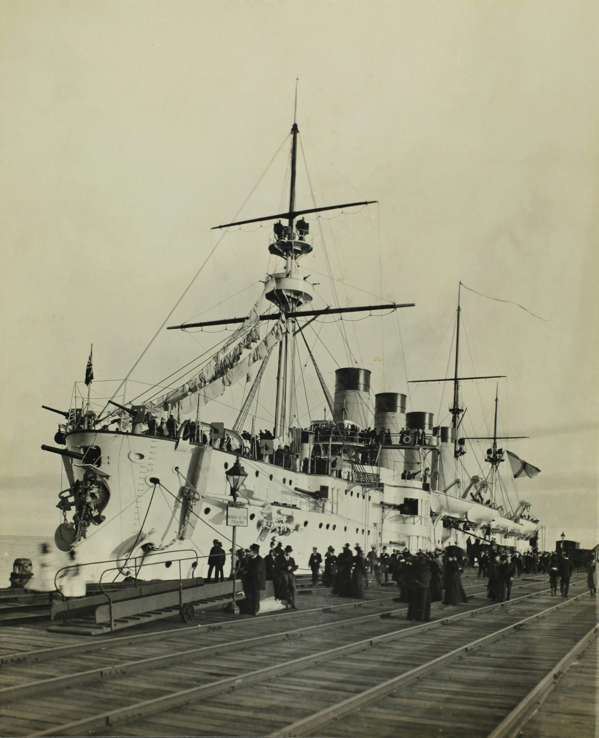
Introduction

Titanic shipwreck was a serious historic incident that formed how we view human survival throughout disasters. Even a century later, this tragic incident nonetheless gives useful insights and classes.

The RMS Titanic was one of many largest and most luxurious ship of its time. It was nicknamed “The Unsinkable” by its proud makers. On April tenth, 1912, it set out on its first journey from England to New York. The Titanic took with all of it courses of individuals, the rich and the poor. It was commanded by the Senior Captain Edward John Smith. Throughout the course of its voyage, the Titanic obtained a number of warnings of ice on the Atlantic, which made it change its course twice. However on the 4th day of its voyage, 14th April, it collided with an enormous iceberg that led to the start of the gradual sinking of this luxury ship. The ship despatched radio alerts to different close by ships for assist, however solely one in all them responded. The captain ordered the passengers to be evacuated. Based on the protocol, the ladies and youngsters had been to be evacuated first utilizing the lifeboats obtainable on the ship. However as we are going to see in our explorations, it didn’t actually occur as such. Sure different components additionally performed a job in figuring out the survival of the passengers aboard. It appeared as if some teams of individuals had been extra prone to survive than others, and that is what we are going to discover on this article.

The sinking of this “Unsinkable” ship prompted the loss of life of 1502 out of 2224 of its passengers and crew.

The Challenge

Titanic dataset is a really beginner-friendly dataset, and that’s the reason it’s broadly used as the place to begin in knowledge science studying. Not solely does it present attention-grabbing patterns for knowledge analytics, nevertheless it retains its worth in combining each historic context with actual human decision-making below disaster circumstances.

On this article, we are going to do an exploratory knowledge evaluation of the Titanic Dataset. We’ll see what the info appears like, what the completely different attributes are at play, and the way these completely different attributes affected the survival of the passenger. This can be a beginner-friendly tutorial that requires a primary understanding of Python fundamentals, importing libraries and using its capabilities for knowledge evaluation. By combining knowledge storytelling and sample recognition, to the earlier articles and initiatives on it by means of its insights as to how social inequality, evacuation habits, and household construction affect survival outcomes.

The Dataset

On this tutorial, we are going to entry the Titanic dataset and use Python pandas, matplotlib, and seaborn to discover how various factors performed a job within the survival of the passengers. Allow us to obtain and cargo the info in order that it’s accessible in our code.

You will get the dataset from the : Github Hyperlink

Loading the Dataset

After getting the info URL, you’ll be able to entry it as a pandas dataframe. We should set up/import pandas for this. Pandas is a robust Python library for knowledge evaluation and manipulation. If not already put in in your IDE, set up it from the terminal by means of pip as follows:

pip set up pandas

As soon as the set up is full, import the library in your Python file by aliasing it as pd:

import pandas as pd

Subsequent, learn the info utilizing the Pandas read_csv perform. Be sure to add the URL as observe:

url = "https://uncooked.githubusercontent.com/datasciencedojo/datasets/grasp/titanic.csv"

df = pd.read_csv(url)

This can load the file as a pandas dataframe within the variable “df”. We’ll do the info evaluation and exploration utilizing this dataframe that has the info we want saved. Allow us to learn the info on this dataframe utilizing the head() perform that returns the primary 5 traces by default of the dataframe:

print(df.head())

We are able to additionally use the Pandas library’s iloc[0] capabilities to get entry to all of the column names/attributes:

print(df.iloc[0])

Right here we are able to see the primary 5 traces of the dataset, together with the column names. As will be seen within the picture above, the dataset has the next attributes:

1. PassengerId — that is id of the passenger, a numerical worth to establish every passenger
2. Survived — this refers as to if the passenger on board survived the shipwreck or not
3. Pclass — that is concerning the category of the passenger
4. Title — that is the title of the passenger, with applicable titles
5. Intercourse — gender of the passengers
6. Age — age group of the passengers on board
7. SibSp — this refers back to the variety of siblings or spouses on board
8. Parch — this refers back to the variety of mother and father or kids on board
9. Ticket- that is the ticket variety of the passenger 
10. Fare — this refers back to the ticket value 
11. Cabin — that is the cabin variety of the passenger
12. Embarked — this refers to the place the passenger embarked from C = Cherbourg, Q = Queenstown, S = Southampton

As will be seen above, there are a couple of columns or attributes which might be of curiosity to us in figuring out whether or not an individual survived the Titanic or not. Attributes akin to names and ticket quantity don’t appear to affect the survival of passengers. With a view to have a transparent view of this, allow us to do some knowledge evaluation to seek out out the relation between completely different attributes and the way they every affect survival individually and as combos:

Information Evaluation

Earlier than we formally begin the info evaluation, allow us to set up/import the related Python libraries.

The primary one is Matplotlib. This library gives visualization options for knowledge. We’ll plot graphs utilizing this library. The second is Seaborn. Seaborn is a Python knowledge visualization library primarily based on matplotlib, and permits us to create visuals, plots, and figures primarily based on the info. Allow us to set up and import these into our Python file.

pip set up matplotlib
pip set up seaborn

Now import these with alias names simply as we did with the pandas library into the primary coding file.

import seaborn as sns
import matplotlib.pyplot as plt

Now, allow us to see how completely different attributes affected survival:

Describing the Dataset

First allow us to have a generic overview of the info. We’ll use the describe() perform for this. We now have additionally added the pd.set_option to cease knowledge truncation.

pd.set_option('show.max_columns', None)
print(df.describe())

As we are able to see within the picture above, the perform describe() offers a statistical abstract of the whole dataset utilizing metrics like rely, imply, customary deviation, and many others. The data helpful right here is:

• There are a complete of 891 entries of passengers (from rely = 891)
• The survival price is 38% (from the imply of survived = 0.38)
• Most passengers belonged to third class (imply of Pclass = 2.3 nearer to three)
• A number of the passengers’ age knowledge is lacking (the rely of Age isn’t equal to the entries)
• Many of the passengers had been younger (the imply age = 29.6)
• The youngest passenger was 0.4 years (lower than 6 months), and the oldest was 80 years outdated
• The typical ticket value was round £32.38 (imply fare)
• Ticket value different enormously (excessive customary variation for the fare = 49.69)
• Large financial inequality, fare for some was 0, and for others as excessive as £512
• Age quartiles: 25% had been youthful than 20, half had been youthful than 28, and 75% had been youthful than 38

Now that we all know the generic date insights, allow us to deep dive right into a extra detailed evaluation.

Survival Info

First, allow us to do some basic survival evaluation:

survival_counts = df['Survived'].value_counts()
print(survival_counts)

plt.determine(figsize=(6,4))

sns.countplot(
    x='Survived',
    knowledge=df
)

plt.title("Titanic Survival Distribution")

We tapped into the survival attribute and located a rely of 549 for 0, which didn’t survive, and 342 for 1, that’s survived. This can be a 38% survival price as was beforehand obtained from the describe() perform. Now, allow us to transfer to the components that affected this survival.

Survival by Gender

Allow us to see how this survival price was influenced by gender. Did one gender have an edge in survival over the opposite? We all know the priorities had been ladies and youngsters, however what precisely does the info present?

gender_survival = pd.crosstab(
    df['Sex'],
    df['Survived'],
    normalize='index'
)

print(gender_survival)


plt.determine(figsize=(6,4))

sns.barplot(
    x='Intercourse',
    y='Survived',
    knowledge=df
)

plt.title("Survival Charge by Gender")

plt.ylabel("Survival Charge")

plt.present()

As will be seen from each the report and the plot above, the boys’s survival price was simply 18%. Whereas, as a lot as 74% ladies survived the shipwreck.

Survival by Passenger Class

Now, allow us to analyse how passengers from completely different courses survived the incident.

class_survival = pd.crosstab(
    df['Pclass'],
    df['Survived'],
    normalize='index'
)
print(class_survival)

plt.determine(figsize=(7,5))

sns.barplot(
    x='Pclass',
    y='Survived',
    knowledge=df
)

plt.title("Survival Charge by Passenger Class")

plt.xlabel("Passenger Class")

plt.ylabel("Survival Charge")

plt.present()

As will be seen from the report and plot above, about 62% of passengers from the first class survived, 47% from the second class, and solely 24% from the third class. We are able to infer from this very primary plot that the primary class, which paid closely for the ship’s luxuries, has the next probability of survival; they had been most well-liked over the opposite two courses.

Survival by Age

Allow us to see how passengers of various ages survived. Did kids have the next probability of survival?

plt.determine(figsize=(10,6))

sns.histplot(
    knowledge=df,
    x='Age',
    hue='Survived',
    bins=30,
    a number of='stack',
    alpha=0.6
)

plt.title("Age Distribution by Survival")

plt.present()

From this stacked histogram, we are able to draw a number of significant insights about how age is said to survival on the Titanic.

• Most passengers who had been onboard had been younger adults within the age bracket of 20 and 30
• Kids lower than 10 present increased survival illustration with an even bigger orange coloured stack as in comparison with the blue one
• Grownup non-survivors dominated the dataset, with bars representing non-survivors between 20 and 40 being larger
• Survival declines within the older age group; this can be on account of aged passengers going through sure age-restricted challenges in evacuation
• The non-survivor parts of the bars dominate most age ranges, implying that extra passengers died than survived total, aligning with the general survival price of roughly 38%

To summarize, the survival on the Titanic favored youthful passengers, whereas younger grownup populations skilled the best mortality charges.

Kids Precedence

Had been the kids really prioritized? Allow us to reply that with some analytics:

df['IsChild'] = df['Age'] < 16
child_survival = pd.crosstab(
    df['IsChild'],
    df['Survived'],
    normalize='index'
)

print(child_survival)

sns.barplot(
    x='IsChild',
    y='Survived',
    knowledge=df
)

plt.title("Little one vs Grownup Survival")
plt.present()

As will be seen from the above, round 59% of the kids survived, which is a direct reflection of how the kids had been really prioritized.

Now allow us to analyse how household measurement impacted survival.

Household Dimension Evaluation

The household measurement attribute relies on two completely different attributes of the dataset: SibSp and Parch. SibSp is the variety of siblings and spouses of the passenger onboard. Whereas Parch is the variety of mother and father and youngsters of the passenger.

Allow us to see how the household measurement affected survival:

df['FamilySize'] = (
    df['SibSp'] + df['Parch'] + 1
)
plt.determine(figsize=(10,6))

sns.barplot(
    x='FamilySize',
    y='Survived',
    knowledge=df
)

plt.title("Survival Charge by Household Dimension")
plt.present()

The plot above exhibits how survival chance modified relying on the variety of relations touring collectively on the Titanic. The code is easy, it provides the variety of siblings/partner and oldsters/kids, plus the passenger themself because the household measurement. the y-axis of the plot represents the survival chance so every bar exhibits the proportion of passengers with a selected household measurement to have survived. We are able to see from the bar chart above that:

• Passengers touring alone had decrease survival, in all probability becuase the passengers touring alone had much less social assist, no help throughout evacuation, or decrease precedence in comparison with households
• Small households with household sizes of about 2, 3, and 4 had the best survival charges, which can be due to them serving to one another out throughout evacuation, stayed coordinated and obtained precedence in lifeboat boarding
• Very giant households with household measurement better than 6 had decrease survival charges, in all probability on account of issue in coordinating evacuation and households refusing to separate on lifeboats.

As we are able to see, survival was not linearly associated to the household measurement, however a reasonably sized household had the next survival price.

Survival by Fare Paid

Lastly, allow us to see how the ticket value affected survival. We are able to analyse this utilizing a violin plot as beneath:

plt.determine(figsize=(12,6))

sns.violinplot(
    knowledge=df,
    x='Survived',
    y='Fare',
    internal='quartile'
)

plt.xticks(
    [0,1],
    ['Did Not Survive', 'Survived']
)

plt.title(
    "Ticket Fare Distribution by Survival"
)

plt.ylabel("Fare Paid")

plt.present()

The violin plot exhibits a transparent relationship between ticket fare and survival on the Titanic. Survivors typically paid increased fares, whereas most non-survivors had been concentrated in decrease fare ranges. This means that first-class and wealthier passengers had a big survival benefit, seemingly on account of higher cabin places and simpler entry to lifeboats. Nonetheless, the overlap between the 2 teams additionally signifies that wealth alone didn’t decide survival, as components like gender, age, and evacuation timing additionally performed vital roles.

Concluding the Findings

We all know now that sure info like being feminine, a baby, belonging to the primary class, and having a reasonable household measurement performed a job within the passenger’s survival. Allow us to mix these options to find out the survival price.

# CREATE FEATURES

# Little one column
df['IsChild'] = df['Age'] < 16

# Household measurement column
df['FamilySize'] = (
    df['SibSp'] + df['Parch'] + 1
)

# Average household measurement
df['ModerateFamily'] = (
    (df['FamilySize'] >= 2) &
    (df['FamilySize'] <= 4)
)

# Mix all favorable circumstances
combined_condition = (
    (df['Sex'] == 'feminine') &
    (df['Pclass'] == 1) &
    (df['ModerateFamily'] == True)
) | (
    (df['IsChild'] == True)
)

# Create a brand new class column
df['HighSurvivalGroup'] = combined_condition


# PLOT SURVIVAL RATE

plt.determine(figsize=(8,5))

sns.barplot(
    knowledge=df,
    x='HighSurvivalGroup',
    y='Survived'
)

plt.xticks(
    [0,1],
    ['Other Passengers', 'High Survival Group']
)

plt.ylabel("Survival Charge")

plt.title(
    "Survival Charge Primarily based on Mixed Passenger Components"
)

plt.present()

The above code mixed all of the beneficial circumstances for survival and in contrast passengers with these traits
vs everybody else. As will be seen from the graph, the “Excessive Survival Group” had dramatically increased survival charges.

Conclusion

On this article, we’ve efficiently analyzed the Titanic dataset utilizing pandas, matplotlib, and seaborn. That is a simple and beginner-friendly tutorial to grasp how we are able to interpret knowledge, plot graphs, and collect insights from them. From the above findings, we are able to simply group sure options as being beneficial to survival. Furthermore, these knowledge analytics and findings can even assist us in creating an environment friendly machine studying algorithm in predicting the survival of the Titanic passengers.