
A language mannequin doesn’t write textual content immediately. As a substitute, it returns logits for the following token. The decoding algorithm decides easy methods to flip these logits right into a token, and repeating this choice produces the output textual content.
The decoding algorithm impacts the conduct of the mannequin. Grasping decoding is deterministic and steady, however it may be uninteresting. Sampling introduces some randomness, which may produce extra numerous textual content however may produce errors. Beam search will be helpful for some constrained duties however is often not the very best default for chat-style technology. Output constraints could make the mannequin produce JSON or cease at a particular marker.
On this chapter, you’ll study:
- Grasping decoding
- Temperature sampling
- Prime-k and nucleus sampling
- Repetition penalties
- Cease circumstances
- Beam search
- Structured output constraints
Let’s get began.
Decoding Methods and Output Management
Photograph by Claudio Testa. Some rights reserved.
Overview
This chapter is split into 9 components; they’re:
- Studying Logits from a Mannequin
- Grasping Decoding
- Temperature Sampling
- Prime-$ok$ Sampling
- Nucleus Sampling
- Repetition Penalties
- Beam Search
- Cease Situations
- Structured Output Constraints
Studying Logits from a Mannequin
The mannequin returns a vector of logits for each place within the enter sequence. For technology, you usually use solely the final place as a result of it predicts the following token.
The next instance makes use of the Hugging Face transformers library with a small GPT-2 model mannequin. The checkpoint is sufficiently small for native experimentation, however the identical logic applies to bigger fashions.
|
1 2 3 4 5 6 7 8 9 10 11 12 13 14 15 16 17 18 |
import torch from transformers import AutoModelForCausalLM, AutoTokenizer
model_name = “sshleifer/tiny-gpt2” tokenizer = AutoTokenizer.from_pretrained(model_name) mannequin = AutoModelForCausalLM.from_pretrained(model_name) mannequin.eval()
immediate = “A language mannequin is” input_ids = tokenizer(immediate, return_tensors=“pt”).input_ids
with torch.no_grad(): outputs = mannequin(input_ids)
logits = outputs.logits next_token_logits = logits[:, –1, :] print(next_token_logits.form) |
The output form is:
The logits should not chances. To show logits into chances, use softmax:
|
probs = torch.softmax(next_token_logits, dim=–1) |
Nonetheless, you usually don’t have to compute chances explicitly. Grasping decoding solely wants the index of the biggest logit, which is similar because the token with the best likelihood.
|
next_token = next_token_logits.argmax(dim=–1, keepdim=True) print(tokenizer.decode(next_token[0])) |
That is the only decoding technique.
Grasping Decoding
Grasping decoding at all times chooses the token with the best rating. A whole grasping decoding operate will be written as follows:
|
torch.no_grad() def greedy_decode(mannequin, tokenizer, immediate, max_new_tokens=30): input_ids = tokenizer(immediate, return_tensors=“pt”).input_ids
for _ in vary(max_new_tokens): outputs = mannequin(input_ids) next_token_logits = outputs.logits[:, –1, :] next_token = next_token_logits.argmax(dim=–1, keepdim=True) input_ids = torch.cat([input_ids, next_token], dim=1)
if next_token.merchandise() == tokenizer.eos_token_id: break
return tokenizer.decode(input_ids[0], skip_special_tokens=True) |
Grasping decoding is deterministic. Given the identical mannequin and immediate, it returns the identical output. That is helpful for debugging and for duties the place variation is undesirable.
The weak point is that the very best native token just isn’t at all times the very best continuation. Grasping decoding can repeat itself, select frequent phrases too usually, and miss extra fascinating continuations.
Temperature Sampling
Temperature sampling attracts from a likelihood distribution obtained by scaling the logits with a temperature parameter.
The determine beneath exhibits how temperature adjustments the likelihood distribution with out altering the underlying logits. The identical ten token scores are transformed to chances 3 times: as soon as with temperature 0.5, as soon as with temperature 1, and as soon as with temperature 2.
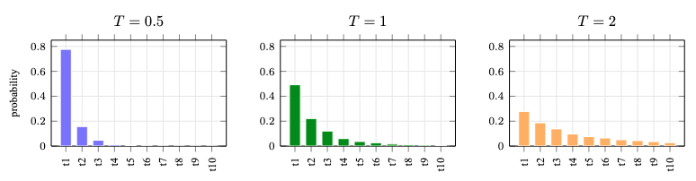
The identical logits produce totally different token chances underneath totally different temperatures. A decrease temperature concentrates likelihood on the highest-scoring token, whereas a better temperature spreads likelihood throughout extra tokens.
Sampling chooses the following token randomly from the mannequin’s likelihood distribution. Temperature controls how sharp or flat that distribution is. Given logits $mathbf{z}$ and temperature $T$, temperature sampling makes use of:
$$
mathbf{p} = operatorname{softmax}(mathbf{z} / T)
$$
A low temperature makes the distribution $mathbf{p}$ sharper. A excessive temperature makes it flatter. If the temperature approaches zero, sampling behaves like grasping decoding, supplied one token has a uniquely highest logit. If the temperature is simply too excessive, variations between the logits turn out to be much less necessary, and the mannequin might select unlikely tokens too usually.
A sampling loop utilizing temperature appears to be like like this:
|
1 2 3 4 5 6 7 8 9 10 11 12 13 14 15 16 17 18 19 |
@torch.no_grad() def temperature_decode(mannequin, tokenizer, immediate, temperature=0.8, max_new_tokens=30): input_ids = tokenizer(immediate, return_tensors=“pt”).input_ids assert temperature > 0, “temperature should be optimistic”
for _ in vary(max_new_tokens): outputs = mannequin(input_ids) # apply temperature to the logits for the following token logits = outputs.logits[:, –1, :] / temperature # convert logits to chances and pattern from the distribution probs = torch.softmax(logits, dim=–1) next_token = torch.multinomial(probs, num_samples=1) # append the following token to the enter for subsequent iteration input_ids = torch.cat([input_ids, next_token], dim=1)
if next_token.merchandise() == tokenizer.eos_token_id: break
return tokenizer.decode(input_ids[0], skip_special_tokens=True) |
Temperature just isn’t a top quality knob by itself. It adjustments the quantity of randomness. The suitable worth depends upon the duty. A factual extraction job often desires a decrease temperature. Brainstorming and artistic writing might profit from a better temperature.
Prime-$ok$ Sampling
Within the determine above, a 10-token distribution is proven for example. An precise mannequin might have a vocabulary of a whole lot of hundreds of tokens, together with many who have extraordinarily low likelihood in a given context.
Prime-$ok$ sampling retains solely the $ok$ highest-scoring tokens and removes all different tokens from consideration. Its main function is to stop the mannequin from sampling extraordinarily unlikely tokens. It doesn’t keep away from computing logits over the complete vocabulary, nevertheless it does cut back the variety of candidates you pattern from.
|
@torch.no_grad() def top_k_sample(logits, ok): assert ok > 0, “ok should be optimistic” assert ok <= logits.measurement(–1), “ok should not exceed the vocabulary measurement”
# Get top-k logits and their indices values, indices = torch.topk(logits, ok) # Convert logits to chances over top-k candidates probs = torch.softmax(values, dim=–1) # Pattern from top-k indices in line with their chances sampled = torch.multinomial(probs, num_samples=1) # Recuperate precise token ids utilizing gathered top-k indices next_token = indices.collect(–1, sampled) return next_token |
Prime-$ok$ is straightforward to know, nevertheless it makes use of a set variety of candidates. Typically the mannequin may be very assured and just a few tokens matter. Typically many tokens are believable, by which case a set top-$ok$ cutoff could also be inappropriate. This motivates nucleus sampling.
Nucleus Sampling
Nucleus sampling, additionally referred to as top-$p$ sampling, retains the smallest set of tokens whose cumulative likelihood is not less than $p$. For instance, with $p=0.9$, it retains the most definitely tokens that collectively account for 90 % of the likelihood mass.
|
1 2 3 4 5 6 7 8 9 10 11 12 13 14 15 16 17 18 19 20 21 22 23 24 25 26 27 28 29 30 31 32 33 34 35 36 37 38 |
torch.no_grad() def top_p_sampling(logits, temperature=1.0, ok=0, p=0.9): “”“ Apply temperature scaling, non-compulsory top-k filtering, and top-p filtering. Settle for a 1D tensor of logits and return one sampled token ID. ““” assert logits.dim() == 1, “logits should be a 1D tensor” assert 0 < p <= 1, “p should be in (0, 1]”
vocab_size = logits.measurement(0)
# Apply temperature logits = logits / temperature
# Optionally available top-k filtering if ok > 0 and ok < vocab_size: topk_vals, topk_idx = torch.topk(logits, ok) # Create a masks crammed with -inf, put top-k logits at their indices new_logits = torch.full_like(logits, float(‘-inf’)) new_logits[topk_idx] = topk_vals logits = new_logits
# Prime-p (nucleus) filtering sorted_logits, sorted_indices = torch.type(logits, descending=True) sorted_probs = torch.softmax(sorted_logits, dim=–1) cumulative_probs = torch.cumsum(sorted_probs, dim=–1)
# Tokens to take away, however preserve not less than one token take away = cumulative_probs > p take away[1:] = take away[:–1].clone() take away[0] = False sorted_logits = sorted_logits.masked_fill(take away, float(‘-inf’))
# Sampling final_probs = torch.softmax(sorted_logits, dim=–1) sampled = torch.multinomial(final_probs, num_samples=1) next_token = sorted_indices.collect(–1, sampled) return next_token |
The operate above combines temperature sampling, non-compulsory top-$ok$ filtering, and top-$p$ filtering. Combining these strategies is frequent. Their order issues as a result of temperature scaling and filtering have an effect on the distribution from which the following token is sampled. Prime-$p$ is adaptive: it might preserve solely a handful of tokens when the mannequin is assured and plenty of tokens when the distribution is broad.
Repetition Penalties
Autoregressive fashions can fall into loops by which a sample of tokens repeats itself. Including a repetition penalty reduces the scores of tokens which have already appeared in order that these tokens are much less more likely to be chosen once more.
One easy model divides optimistic logits by the penalty and multiplies detrimental logits by the penalty:
|
1 2 3 4 5 6 7 8 9 10 11 12 13 14 15 16 17 18 19 20 21 22 23 |
@torch.no_grad() def apply_repetition_penalty(logits, generated_ids, penalty=1.1): assert logits.dim() == 2 and logits.measurement(0) == 1, ( “logits will need to have form [1, vocab_size]” ) assert generated_ids.dim() == 2 and generated_ids.measurement(0) == 1, ( “generated_ids will need to have form [1, sequence_length]” ) assert penalty >= 1.0, “penalty should be not less than 1”
if penalty == 1.0: return logits
logits = logits.clone() token_ids = set(generated_ids[0].tolist()) for token_id in token_ids: token_logit = logits[0, token_id] logits[0, token_id] = torch.the place( token_logit > 0, token_logit / penalty, token_logit * penalty, ) return logits |
This operate is deliberately easy and assumes a batch measurement of 1. For instance, a number of occurrences of the identical token don’t enhance the penalty. The caller additionally decides whether or not generated_ids contains immediate tokens, generated tokens, or each. If you happen to use repetition penalties with top-$ok$ or nucleus sampling, apply the penalties first. Manufacturing implementations often deal with bigger batches and may distinguish frequency penalties from presence penalties.
Repetition penalties may help, however they will additionally hurt high quality. Some phrases ought to repeat. Code, names, citations, and structured codecs usually require precise repetition. Use this management solely when repetition is an actual downside.
Beam Search
Grasping decoding retains just one candidate sequence. Beam search retains a number of candidates. At every step, it expands every candidate with potential subsequent tokens and retains the best-scoring sequences.
Beam search is beneficial when there’s a well-defined sequence-level goal, akin to translation in older sequence-to-sequence methods. For open-ended chat technology, beam search usually produces generic textual content as a result of it favors high-probability continuations.
A minimal beam search loop appears to be like like this:
|
1 2 3 4 5 6 7 8 9 10 11 12 13 14 15 16 17 18 19 20 21 22 23 24 25 26 |
@torch.no_grad() def beam_search(mannequin, tokenizer, immediate, num_beams=3, max_new_tokens=20): input_ids = tokenizer(immediate, return_tensors=“pt”).input_ids beams = [(0.0, input_ids)]
# Every iteration provides one token to every beam for _ in vary(max_new_tokens): candidates = [] # Increase every beam with its num_beams highest-scoring subsequent tokens for rating, token_ids in beams: outputs = mannequin(token_ids) logits = outputs.logits[:, –1, :] log_probs = torch.log_softmax(logits, dim=–1) values, indices = torch.topk(log_probs, num_beams, dim=–1)
for worth, token_id in zip(values[0], indices[0]): next_ids = torch.cat([token_ids, token_id.view(1, 1)], dim=1) candidates.append((rating + worth.merchandise(), next_ids)) # Preserve solely the very best num_beams candidates for the following iteration beams = sorted( candidates, key=lambda candidate: candidate[0], reverse=True )[:num_beams]
# Return solely the very best beam as the ultimate output best_score, best_token_ids = beams[0] return tokenizer.decode(best_token_ids[0], skip_special_tokens=True) |
This implementation is intentionally small. An actual implementation ought to normalize scores by sequence size, deal with end-of-sequence tokens, and keep away from recomputing the entire prefix by utilizing a KV cache.
Beam search is pricey: the loops make technology slower, and the variety of beams will increase reminiscence utilization. If you happen to use 4 beams, the mannequin tracks 4 continuations. This will increase compute and cache reminiscence in contrast with bizarre sampling. Subsequently, beam search is often averted in LLM companies.
Cease Situations
Technology should cease in some unspecified time in the future. The only cease situation is a most variety of new tokens. One other frequent situation is the mannequin’s end-of-sequence token. Often the vocabulary in a language mannequin incorporates some particular tokens. The top-of-sequence token is one among them.
The grasping decoding instance above will be modified to simply accept an arbitrary cease token:
|
@torch.no_grad() def greedy_decode_with_stop(mannequin, tokenizer, immediate, stop_token_id, max_new_tokens=30): input_ids = tokenizer(immediate, return_tensors=“pt”).input_ids
for _ in vary(max_new_tokens): outputs = mannequin(input_ids) next_token_logits = outputs.logits[:, –1, :] next_token = next_token_logits.argmax(dim=–1, keepdim=True) input_ids = torch.cat([input_ids, next_token], dim=1)
if next_token.merchandise() == stop_token_id: break
return tokenizer.decode(input_ids[0], skip_special_tokens=True) |
This operate checks whether or not the following token is the cease token. Whether it is, the loop ends and the operate returns the generated textual content earlier than reaching the utmost variety of new tokens. This implementation doesn’t deal with batched inputs; it assumes a single immediate. With batched inputs, totally different sequences might cease at totally different occasions, by which case extra subtle dealing with is required.
Structured Output Constraints
Some purposes want the mannequin to supply a format akin to JSON, a SQL question, or a price from a set listing. One method is to immediate the mannequin and *hope* that it follows the format. A stronger method is constrained decoding.
The concept is to masks out tokens that will make the output invalid. For instance, if the output should be one among three labels, you’ll be able to rating solely these labels:
|
1 2 3 4 5 6 7 8 9 10 11 12 13 14 15 16 17 18 19 |
@torch.no_grad() def choose_label(mannequin, tokenizer, immediate, labels): assert labels, “labels should not be empty”
# Run the immediate to acquire logits over the vocabulary input_ids = tokenizer(immediate, return_tensors=“pt”).input_ids outputs = mannequin(input_ids) logits = outputs.logits[:, –1, :]
# Rating every label, assuming that it’s precisely one token on this context label_scores = [] for label in labels: # Embody any required main whitespace within the label string label_ids = tokenizer.encode(label, add_special_tokens=False) assert len(label_ids) == 1, f“{label!r} should encode to precisely one token” label_scores.append(logits[0, label_ids[0]].merchandise())
best_score, best_label = max(zip(label_scores, labels)) return best_label |
This instance handles solely labels that encode to 1 token after the immediate. Tokenization can rely upon context, together with previous whitespace, so callers should assemble the labels accordingly. Multi-token labels require scoring full token sequences or constraining every decoding step. Structured decoding turns output necessities into token constraints. Extra superior methods use grammars, tries, or finite-state machines to determine which tokens are legitimate at every step.
Constrained decoding can enhance reliability, however it could possibly additionally gradual inference. The system should compute and apply token masks at every step. As with each inference approach, it is best to measure each high quality and efficiency.
Additional Studying
Under are some assets it’s possible you’ll discover helpful:
- Softmax operate, on Wikipedia.
This can be a helpful reference for a way logits are transformed into chances. Temperature sampling is a direct modification of the softmax enter, changing $mathbf{z}$ with $mathbf{z}/T$ earlier than normalization. - Beam search, on Wikipedia.
This web page describes beam search as a basic heuristic search algorithm. In language technology, beam search retains a number of candidate continuations as a substitute of solely the only greatest subsequent token. - The Curious Case of Neural Textual content Degeneration, by Holtzman et al.
This paper explains why maximum-likelihood decoding strategies akin to grasping decoding and beam search can produce bland or repetitive textual content, and introduces nucleus sampling as a sensible various for open-ended technology. - Contrastive Decoding: Open-ended Textual content Technology as Optimization, by Li et al.
This paper proposes a decoding methodology that compares an skilled language mannequin with a smaller novice mannequin, utilizing the distinction between their scores to want fluent and informative continuations. - Grammar-Constrained Decoding for Structured NLP Duties with out Finetuning, by Geng et al.
This paper discusses how formal grammars can constrain the token selections of a language mannequin in order that generated outputs comply with a required construction. - Producing Structured Outputs from Language Fashions: Benchmark and Research, by Geng et al.
This paper research constrained decoding for structured outputs akin to JSON schemas, and is particularly related when the objective is dependable machine-readable output moderately than free-form textual content.
Abstract
On this chapter, you realized that decoding is the method of selecting tokens from logits. Grasping decoding is deterministic and easy. Temperature sampling, top-$ok$ sampling, and nucleus sampling introduce managed randomness. Beam search tracks a number of candidates however will increase inference price. Repetition penalties and cease circumstances assist management output size and conduct. Structured output constraints could make mannequin outputs simpler to make use of in purposes.
Within the subsequent chapter, you’ll discover ways to measure inference efficiency in order that these selections will be in contrast with actual numbers as a substitute of instinct.
A language mannequin doesn’t write textual content immediately. As a substitute, it returns logits for the following token. The decoding algorithm decides easy methods to flip these logits right into a token, and repeating this choice produces the output textual content.
The decoding algorithm impacts the conduct of the mannequin. Grasping decoding is deterministic and steady, however it may be uninteresting. Sampling introduces some randomness, which may produce extra numerous textual content however may produce errors. Beam search will be helpful for some constrained duties however is often not the very best default for chat-style technology. Output constraints could make the mannequin produce JSON or cease at a particular marker.
On this chapter, you’ll study:
- Grasping decoding
- Temperature sampling
- Prime-k and nucleus sampling
- Repetition penalties
- Cease circumstances
- Beam search
- Structured output constraints
Let’s get began.
Decoding Methods and Output Management
Photograph by Claudio Testa. Some rights reserved.
Overview
This chapter is split into 9 components; they’re:
- Studying Logits from a Mannequin
- Grasping Decoding
- Temperature Sampling
- Prime-$ok$ Sampling
- Nucleus Sampling
- Repetition Penalties
- Beam Search
- Cease Situations
- Structured Output Constraints
Studying Logits from a Mannequin
The mannequin returns a vector of logits for each place within the enter sequence. For technology, you usually use solely the final place as a result of it predicts the following token.
The next instance makes use of the Hugging Face transformers library with a small GPT-2 model mannequin. The checkpoint is sufficiently small for native experimentation, however the identical logic applies to bigger fashions.
|
1 2 3 4 5 6 7 8 9 10 11 12 13 14 15 16 17 18 |
import torch from transformers import AutoModelForCausalLM, AutoTokenizer
model_name = “sshleifer/tiny-gpt2” tokenizer = AutoTokenizer.from_pretrained(model_name) mannequin = AutoModelForCausalLM.from_pretrained(model_name) mannequin.eval()
immediate = “A language mannequin is” input_ids = tokenizer(immediate, return_tensors=“pt”).input_ids
with torch.no_grad(): outputs = mannequin(input_ids)
logits = outputs.logits next_token_logits = logits[:, –1, :] print(next_token_logits.form) |
The output form is:
The logits should not chances. To show logits into chances, use softmax:
|
probs = torch.softmax(next_token_logits, dim=–1) |
Nonetheless, you usually don’t have to compute chances explicitly. Grasping decoding solely wants the index of the biggest logit, which is similar because the token with the best likelihood.
|
next_token = next_token_logits.argmax(dim=–1, keepdim=True) print(tokenizer.decode(next_token[0])) |
That is the only decoding technique.
Grasping Decoding
Grasping decoding at all times chooses the token with the best rating. A whole grasping decoding operate will be written as follows:
|
torch.no_grad() def greedy_decode(mannequin, tokenizer, immediate, max_new_tokens=30): input_ids = tokenizer(immediate, return_tensors=“pt”).input_ids
for _ in vary(max_new_tokens): outputs = mannequin(input_ids) next_token_logits = outputs.logits[:, –1, :] next_token = next_token_logits.argmax(dim=–1, keepdim=True) input_ids = torch.cat([input_ids, next_token], dim=1)
if next_token.merchandise() == tokenizer.eos_token_id: break
return tokenizer.decode(input_ids[0], skip_special_tokens=True) |
Grasping decoding is deterministic. Given the identical mannequin and immediate, it returns the identical output. That is helpful for debugging and for duties the place variation is undesirable.
The weak point is that the very best native token just isn’t at all times the very best continuation. Grasping decoding can repeat itself, select frequent phrases too usually, and miss extra fascinating continuations.
Temperature Sampling
Temperature sampling attracts from a likelihood distribution obtained by scaling the logits with a temperature parameter.
The determine beneath exhibits how temperature adjustments the likelihood distribution with out altering the underlying logits. The identical ten token scores are transformed to chances 3 times: as soon as with temperature 0.5, as soon as with temperature 1, and as soon as with temperature 2.
The identical logits produce totally different token chances underneath totally different temperatures. A decrease temperature concentrates likelihood on the highest-scoring token, whereas a better temperature spreads likelihood throughout extra tokens.
Sampling chooses the following token randomly from the mannequin’s likelihood distribution. Temperature controls how sharp or flat that distribution is. Given logits $mathbf{z}$ and temperature $T$, temperature sampling makes use of:
$$
mathbf{p} = operatorname{softmax}(mathbf{z} / T)
$$
A low temperature makes the distribution $mathbf{p}$ sharper. A excessive temperature makes it flatter. If the temperature approaches zero, sampling behaves like grasping decoding, supplied one token has a uniquely highest logit. If the temperature is simply too excessive, variations between the logits turn out to be much less necessary, and the mannequin might select unlikely tokens too usually.
A sampling loop utilizing temperature appears to be like like this:
|
1 2 3 4 5 6 7 8 9 10 11 12 13 14 15 16 17 18 19 |
@torch.no_grad() def temperature_decode(mannequin, tokenizer, immediate, temperature=0.8, max_new_tokens=30): input_ids = tokenizer(immediate, return_tensors=“pt”).input_ids assert temperature > 0, “temperature should be optimistic”
for _ in vary(max_new_tokens): outputs = mannequin(input_ids) # apply temperature to the logits for the following token logits = outputs.logits[:, –1, :] / temperature # convert logits to chances and pattern from the distribution probs = torch.softmax(logits, dim=–1) next_token = torch.multinomial(probs, num_samples=1) # append the following token to the enter for subsequent iteration input_ids = torch.cat([input_ids, next_token], dim=1)
if next_token.merchandise() == tokenizer.eos_token_id: break
return tokenizer.decode(input_ids[0], skip_special_tokens=True) |
Temperature just isn’t a top quality knob by itself. It adjustments the quantity of randomness. The suitable worth depends upon the duty. A factual extraction job often desires a decrease temperature. Brainstorming and artistic writing might profit from a better temperature.
Prime-$ok$ Sampling
Within the determine above, a 10-token distribution is proven for example. An precise mannequin might have a vocabulary of a whole lot of hundreds of tokens, together with many who have extraordinarily low likelihood in a given context.
Prime-$ok$ sampling retains solely the $ok$ highest-scoring tokens and removes all different tokens from consideration. Its main function is to stop the mannequin from sampling extraordinarily unlikely tokens. It doesn’t keep away from computing logits over the complete vocabulary, nevertheless it does cut back the variety of candidates you pattern from.
|
@torch.no_grad() def top_k_sample(logits, ok): assert ok > 0, “ok should be optimistic” assert ok <= logits.measurement(–1), “ok should not exceed the vocabulary measurement”
# Get top-k logits and their indices values, indices = torch.topk(logits, ok) # Convert logits to chances over top-k candidates probs = torch.softmax(values, dim=–1) # Pattern from top-k indices in line with their chances sampled = torch.multinomial(probs, num_samples=1) # Recuperate precise token ids utilizing gathered top-k indices next_token = indices.collect(–1, sampled) return next_token |
Prime-$ok$ is straightforward to know, nevertheless it makes use of a set variety of candidates. Typically the mannequin may be very assured and just a few tokens matter. Typically many tokens are believable, by which case a set top-$ok$ cutoff could also be inappropriate. This motivates nucleus sampling.
Nucleus Sampling
Nucleus sampling, additionally referred to as top-$p$ sampling, retains the smallest set of tokens whose cumulative likelihood is not less than $p$. For instance, with $p=0.9$, it retains the most definitely tokens that collectively account for 90 % of the likelihood mass.
|
1 2 3 4 5 6 7 8 9 10 11 12 13 14 15 16 17 18 19 20 21 22 23 24 25 26 27 28 29 30 31 32 33 34 35 36 37 38 |
torch.no_grad() def top_p_sampling(logits, temperature=1.0, ok=0, p=0.9): “”“ Apply temperature scaling, non-compulsory top-k filtering, and top-p filtering. Settle for a 1D tensor of logits and return one sampled token ID. ““” assert logits.dim() == 1, “logits should be a 1D tensor” assert 0 < p <= 1, “p should be in (0, 1]”
vocab_size = logits.measurement(0)
# Apply temperature logits = logits / temperature
# Optionally available top-k filtering if ok > 0 and ok < vocab_size: topk_vals, topk_idx = torch.topk(logits, ok) # Create a masks crammed with -inf, put top-k logits at their indices new_logits = torch.full_like(logits, float(‘-inf’)) new_logits[topk_idx] = topk_vals logits = new_logits
# Prime-p (nucleus) filtering sorted_logits, sorted_indices = torch.type(logits, descending=True) sorted_probs = torch.softmax(sorted_logits, dim=–1) cumulative_probs = torch.cumsum(sorted_probs, dim=–1)
# Tokens to take away, however preserve not less than one token take away = cumulative_probs > p take away[1:] = take away[:–1].clone() take away[0] = False sorted_logits = sorted_logits.masked_fill(take away, float(‘-inf’))
# Sampling final_probs = torch.softmax(sorted_logits, dim=–1) sampled = torch.multinomial(final_probs, num_samples=1) next_token = sorted_indices.collect(–1, sampled) return next_token |
The operate above combines temperature sampling, non-compulsory top-$ok$ filtering, and top-$p$ filtering. Combining these strategies is frequent. Their order issues as a result of temperature scaling and filtering have an effect on the distribution from which the following token is sampled. Prime-$p$ is adaptive: it might preserve solely a handful of tokens when the mannequin is assured and plenty of tokens when the distribution is broad.
Repetition Penalties
Autoregressive fashions can fall into loops by which a sample of tokens repeats itself. Including a repetition penalty reduces the scores of tokens which have already appeared in order that these tokens are much less more likely to be chosen once more.
One easy model divides optimistic logits by the penalty and multiplies detrimental logits by the penalty:
|
1 2 3 4 5 6 7 8 9 10 11 12 13 14 15 16 17 18 19 20 21 22 23 |
@torch.no_grad() def apply_repetition_penalty(logits, generated_ids, penalty=1.1): assert logits.dim() == 2 and logits.measurement(0) == 1, ( “logits will need to have form [1, vocab_size]” ) assert generated_ids.dim() == 2 and generated_ids.measurement(0) == 1, ( “generated_ids will need to have form [1, sequence_length]” ) assert penalty >= 1.0, “penalty should be not less than 1”
if penalty == 1.0: return logits
logits = logits.clone() token_ids = set(generated_ids[0].tolist()) for token_id in token_ids: token_logit = logits[0, token_id] logits[0, token_id] = torch.the place( token_logit > 0, token_logit / penalty, token_logit * penalty, ) return logits |
This operate is deliberately easy and assumes a batch measurement of 1. For instance, a number of occurrences of the identical token don’t enhance the penalty. The caller additionally decides whether or not generated_ids contains immediate tokens, generated tokens, or each. If you happen to use repetition penalties with top-$ok$ or nucleus sampling, apply the penalties first. Manufacturing implementations often deal with bigger batches and may distinguish frequency penalties from presence penalties.
Repetition penalties may help, however they will additionally hurt high quality. Some phrases ought to repeat. Code, names, citations, and structured codecs usually require precise repetition. Use this management solely when repetition is an actual downside.
Beam Search
Grasping decoding retains just one candidate sequence. Beam search retains a number of candidates. At every step, it expands every candidate with potential subsequent tokens and retains the best-scoring sequences.
Beam search is beneficial when there’s a well-defined sequence-level goal, akin to translation in older sequence-to-sequence methods. For open-ended chat technology, beam search usually produces generic textual content as a result of it favors high-probability continuations.
A minimal beam search loop appears to be like like this:
|
1 2 3 4 5 6 7 8 9 10 11 12 13 14 15 16 17 18 19 20 21 22 23 24 25 26 |
@torch.no_grad() def beam_search(mannequin, tokenizer, immediate, num_beams=3, max_new_tokens=20): input_ids = tokenizer(immediate, return_tensors=“pt”).input_ids beams = [(0.0, input_ids)]
# Every iteration provides one token to every beam for _ in vary(max_new_tokens): candidates = [] # Increase every beam with its num_beams highest-scoring subsequent tokens for rating, token_ids in beams: outputs = mannequin(token_ids) logits = outputs.logits[:, –1, :] log_probs = torch.log_softmax(logits, dim=–1) values, indices = torch.topk(log_probs, num_beams, dim=–1)
for worth, token_id in zip(values[0], indices[0]): next_ids = torch.cat([token_ids, token_id.view(1, 1)], dim=1) candidates.append((rating + worth.merchandise(), next_ids)) # Preserve solely the very best num_beams candidates for the following iteration beams = sorted( candidates, key=lambda candidate: candidate[0], reverse=True )[:num_beams]
# Return solely the very best beam as the ultimate output best_score, best_token_ids = beams[0] return tokenizer.decode(best_token_ids[0], skip_special_tokens=True) |
This implementation is intentionally small. An actual implementation ought to normalize scores by sequence size, deal with end-of-sequence tokens, and keep away from recomputing the entire prefix by utilizing a KV cache.
Beam search is pricey: the loops make technology slower, and the variety of beams will increase reminiscence utilization. If you happen to use 4 beams, the mannequin tracks 4 continuations. This will increase compute and cache reminiscence in contrast with bizarre sampling. Subsequently, beam search is often averted in LLM companies.
Cease Situations
Technology should cease in some unspecified time in the future. The only cease situation is a most variety of new tokens. One other frequent situation is the mannequin’s end-of-sequence token. Often the vocabulary in a language mannequin incorporates some particular tokens. The top-of-sequence token is one among them.
The grasping decoding instance above will be modified to simply accept an arbitrary cease token:
|
@torch.no_grad() def greedy_decode_with_stop(mannequin, tokenizer, immediate, stop_token_id, max_new_tokens=30): input_ids = tokenizer(immediate, return_tensors=“pt”).input_ids
for _ in vary(max_new_tokens): outputs = mannequin(input_ids) next_token_logits = outputs.logits[:, –1, :] next_token = next_token_logits.argmax(dim=–1, keepdim=True) input_ids = torch.cat([input_ids, next_token], dim=1)
if next_token.merchandise() == stop_token_id: break
return tokenizer.decode(input_ids[0], skip_special_tokens=True) |
This operate checks whether or not the following token is the cease token. Whether it is, the loop ends and the operate returns the generated textual content earlier than reaching the utmost variety of new tokens. This implementation doesn’t deal with batched inputs; it assumes a single immediate. With batched inputs, totally different sequences might cease at totally different occasions, by which case extra subtle dealing with is required.
Structured Output Constraints
Some purposes want the mannequin to supply a format akin to JSON, a SQL question, or a price from a set listing. One method is to immediate the mannequin and *hope* that it follows the format. A stronger method is constrained decoding.
The concept is to masks out tokens that will make the output invalid. For instance, if the output should be one among three labels, you’ll be able to rating solely these labels:
|
1 2 3 4 5 6 7 8 9 10 11 12 13 14 15 16 17 18 19 |
@torch.no_grad() def choose_label(mannequin, tokenizer, immediate, labels): assert labels, “labels should not be empty”
# Run the immediate to acquire logits over the vocabulary input_ids = tokenizer(immediate, return_tensors=“pt”).input_ids outputs = mannequin(input_ids) logits = outputs.logits[:, –1, :]
# Rating every label, assuming that it’s precisely one token on this context label_scores = [] for label in labels: # Embody any required main whitespace within the label string label_ids = tokenizer.encode(label, add_special_tokens=False) assert len(label_ids) == 1, f“{label!r} should encode to precisely one token” label_scores.append(logits[0, label_ids[0]].merchandise())
best_score, best_label = max(zip(label_scores, labels)) return best_label |
This instance handles solely labels that encode to 1 token after the immediate. Tokenization can rely upon context, together with previous whitespace, so callers should assemble the labels accordingly. Multi-token labels require scoring full token sequences or constraining every decoding step. Structured decoding turns output necessities into token constraints. Extra superior methods use grammars, tries, or finite-state machines to determine which tokens are legitimate at every step.
Constrained decoding can enhance reliability, however it could possibly additionally gradual inference. The system should compute and apply token masks at every step. As with each inference approach, it is best to measure each high quality and efficiency.
Additional Studying
Under are some assets it’s possible you’ll discover helpful:
- Softmax operate, on Wikipedia.
This can be a helpful reference for a way logits are transformed into chances. Temperature sampling is a direct modification of the softmax enter, changing $mathbf{z}$ with $mathbf{z}/T$ earlier than normalization. - Beam search, on Wikipedia.
This web page describes beam search as a basic heuristic search algorithm. In language technology, beam search retains a number of candidate continuations as a substitute of solely the only greatest subsequent token. - The Curious Case of Neural Textual content Degeneration, by Holtzman et al.
This paper explains why maximum-likelihood decoding strategies akin to grasping decoding and beam search can produce bland or repetitive textual content, and introduces nucleus sampling as a sensible various for open-ended technology. - Contrastive Decoding: Open-ended Textual content Technology as Optimization, by Li et al.
This paper proposes a decoding methodology that compares an skilled language mannequin with a smaller novice mannequin, utilizing the distinction between their scores to want fluent and informative continuations. - Grammar-Constrained Decoding for Structured NLP Duties with out Finetuning, by Geng et al.
This paper discusses how formal grammars can constrain the token selections of a language mannequin in order that generated outputs comply with a required construction. - Producing Structured Outputs from Language Fashions: Benchmark and Research, by Geng et al.
This paper research constrained decoding for structured outputs akin to JSON schemas, and is particularly related when the objective is dependable machine-readable output moderately than free-form textual content.
Abstract
On this chapter, you realized that decoding is the method of selecting tokens from logits. Grasping decoding is deterministic and easy. Temperature sampling, top-$ok$ sampling, and nucleus sampling introduce managed randomness. Beam search tracks a number of candidates however will increase inference price. Repetition penalties and cease circumstances assist management output size and conduct. Structured output constraints could make mannequin outputs simpler to make use of in purposes.
Within the subsequent chapter, you’ll discover ways to measure inference efficiency in order that these selections will be in contrast with actual numbers as a substitute of instinct.