When Labels Say No, However Embeddings Say Sure

“There may be nothing extra misleading than an apparent reality.”
— Sherlock Holmes, in “The Boscombe Valley Thriller” by Arthur Conan Doyle

1. Introduction

You simply gained the lottery, and your first buy will fulfill a childhood dream: shopping for a Ferrari. You go to a luxurious automobile web site, discover a beautiful Ferrari sports activities automobile, and click on “Discover Related.” The outcomes? 4 Ferraris (nice!), one Lamborghini (cool!), and a Ferrari SUV (wait, what?). You’re keen on the Ferrari and Lamborghini suggestions. However the Ferrari SUV? That is means off from what you had in thoughts.

Why did the Lamborghini seem? As a result of it shares the visible traits that attracted you to the Ferrari: comparable low profile, clean curves, and sporty design. And the Ferrari SUV? Maybe the retrieval system gave a big weight to traits related to the Ferrari model, regardless of its very completely different form. Each outcomes replicate similarity, however two very completely different notions of what it means to be comparable.

Now comes the fascinating half.

Suppose the search engine is evaluated utilizing a benchmark that considers two automobiles related provided that they share the identical model label. The Lamborghini can be counted as a mistake, whereas the Ferrari SUV would obtain full credit score.

So the automobile you’re keen on is fallacious, and the automobile you do not need is true. One thing appears a bit backward right here, does not it?

This instance reveals a giant limitation of category-based retrieval analysis: semantic similarity and categorical settlement aren’t essentially the identical. A retrieval system could uncover significant relationships between objects from completely different classes, however get a penalty simply because their labels do not match.

This raises an intriguing query:

When embeddings discover significant similarities that labels fail to acknowledge, ought to we actually name these retrievals errors?

On this article, we examine this query utilizing CLIP (Contrastive Language–Picture Pre-training), one of the vital well-known vision-language fashions for representing pictures and textual content in a shared embedding area.

Our experiment makes use of a Kaggle dataset containing 9,315 pictures throughout 23 architectural types. Why structure? As a result of buildings from completely different architectural types can have comparable roofs, home windows, supplies, symmetry, and ornamental particulars. Two buildings can look very comparable with out having the identical architectural label.

This can be a excellent case for investigating whether or not CLIP is really confused—or whether or not our analysis standards are typically too inflexible.

1.1 What We Will Discover

We start by explaining how CLIP represents pictures as embeddings and measures similarity utilizing cosine similarity.

Subsequent, we introduce our architectural picture dataset and set up CLIP’s baseline retrieval efficiency utilizing the next: Precision@1, Precision@5, and Precision@10.

Precision@ok (P@ok) measures the proportion of the highest ok retrieved pictures which might be related to the question. In our experiments, a picture is taken into account related if it has the identical architectural model label because the question picture. For instance, a Precision@5 of 0.80 signifies that 4 of the 5 highest-ranked retrieved pictures belong to the identical architectural model because the question.

We then transcend class labels and measure architectural similarity utilizing roof sorts, supplies, symmetry, home windows, and different distinctive options.

We then take a more in-depth have a look at CLIP’s obvious errors, which we name label mismatches. Are these mismatches random, or does CLIP are inclined to retrieve architecturally associated types? We have a look at similarity scores, frequent mismatches, and the way architectural types are associated.

Lastly, we take into account what all this implies for retrieval analysis. Ought to relevance be a easy sure or no, or can measuring levels of similarity give us a greater image of retrieval high quality?

Our objective is to not show that CLIP is at all times proper. Some errors are simply errors. However maybe others deserve a re-assessment.

In spite of everything, in case you requested for a Ferrari sports activities automobile and obtained a Lamborghini, would you actually complain?

2. How CLIP Sees Similarity

As soon as we now have the embeddings, we’d like a mathematical technique to evaluate them.

One of the vital extensively used measures is cosine similarity:

Cosine similarity measures the angle between two vectors relatively than their absolute lengths. A worth of 1 signifies the vectors level in the identical course, whereas 0 signifies they’re orthogonal.

In our retrieval pipeline, we normalize the embeddings and rank candidate pictures by their cosine similarity to the question embedding. The result’s a ranked record of pictures in response to their proximity in CLIP‘s realized illustration.

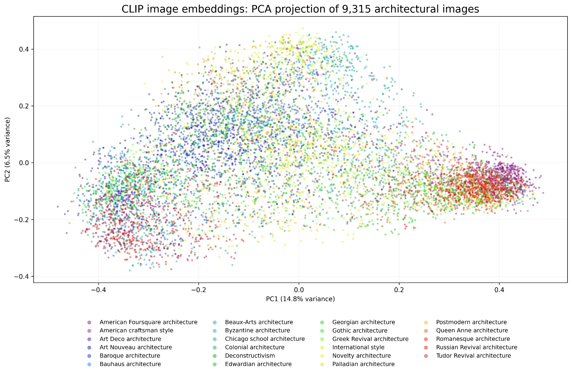
To get a glimpse of this high-dimensional area, we use Principal Part Evaluation (PCA) to venture CLIP’s 512-dimensional picture embeddings onto two dimensions.

The PCA projection of CLIP’s picture embeddings reveals some clustering by architectural model, but in addition appreciable overlap between completely different types. Nevertheless, the primary two principal parts clarify solely 21.3% of the overall variance. Due to this fact, the two-dimensional projection captures solely a small portion of the knowledge within the authentic 512-dimensional embedding area, and the obvious overlap needs to be interpreted with warning.

Up to now, so good. However discover one thing necessary:

Cosine similarity tells us how shut two pictures are in CLIP’s embedding area. It doesn’t inform us which traits produced that similarity—or whether or not these traits are related to the consumer’s search.

CLIP’s embeddings seize details about objects, their look, composition, and that means. Nevertheless, the mannequin doesn’t inform us how a lot every of those components contributes to a similarity rating.

This distinction issues as a result of two pictures may be shut in embedding area for causes which have little to do with the traits we really care about.

2.2 Once we get a label mismatch

Think about a picture of a Gothic constructing submitted as a question. Suppose CLIP retrieves one other Gothic constructing as its closest match. Glorious! A label-based benchmark offers it full credit score.

Now suppose it retrieves a Romanesque constructing as a substitute. The benchmark marks the end result as incorrect as a result of the architectural labels differ. However Gothic and Romanesque buildings have a lot in frequent, together with stone development, arches, heavy structural parts, and historic influences.

Might CLIP have captured a significant architectural relationship? Presumably.

After all, not each label mismatch is a hidden success. Generally CLIP could retrieve a constructing due to its background, lighting, photographic perspective, or different traits unrelated to architectural model.

We wish to discover out whether or not CLIP’s label mismatches replicate actual similarities between architectural types or simply coincidental ones. To do that, we have to transcend appropriate and incorrect labels and measure how a lot architectural types have in frequent.

And that brings us to our experiment.

3. From Ferraris to Facades: Our Architectural Experiment

Architectural types usually share traits, so we are able to look at whether or not CLIP’s label mismatches replicate significant similarities relatively than arbitrary retrievals.

3.1 The Dataset

We started with a Kaggle architectural picture dataset containing 10,113 pictures representing 25 architectural types. We excluded two classes—Achaemenid and Historical Egyptian structure—as a result of they primarily embody historical monuments, whereas our search system focuses on homes and comparable buildings. After eradicating these classes, our remaining dataset contained 9,315 pictures throughout 23 architectural types.

The gathering consists of Gothic, Romanesque, Bauhaus, Worldwide, Georgian, Greek Revival, Artwork Deco, and different architectural types. Every picture has an architectural-style label, permitting us to judge retrieval efficiency utilizing typical category-based metrics.

However we wish to go additional.

When CLIP retrieves a picture from a special architectural model, we wish to know whether or not the question and retrieved types share significant architectural traits. For that, we’d like a further supply of data past CLIP’s embeddings and the dataset’s labels.

3.2 Two Methods to Choose a Retrieval

We consider CLIP from two complementary views.

First: Categorical relevance.

That is the traditional strategy. A retrieved picture is taken into account related if its architectural-style label matches the question’s label. We calculate Precision@1, Precision@5, and Precision@10 to ascertain our baseline. These metrics inform us how successfully CLIP retrieves pictures belonging to the identical labeled architectural class.

Second: Architectural similarity.

Right here, we glance past the labels.

We assemble a structured illustration of architectural traits, together with roof sorts, supplies, symmetry, window configurations, and distinctive options. Utilizing these traits, we calculate a similarity measure between architectural types.

This offers us an unbiased technique to examine whether or not label-mismatched retrievals are inclined to contain types that share architectural options. You will need to observe that our measure compares architectural types primarily based on their frequent options. It doesn’t evaluate particular person buildings. Buildings from associated architectural types should look very completely different.

Our goal is to not declare each label mismatch appropriate, nor to exchange typical retrieval metrics. As a substitute, we wish to look at what these metrics is likely to be lacking.

4. The Baseline: How Usually Does CLIP Get It Proper?

Earlier than questioning whether or not CLIP’s errors are actually errors, we have to set up how nicely it performs in response to typical retrieval metrics.

Our experiment makes use of 9,315 pictures representing 23 architectural types. Every picture serves as a question, and CLIP retrieves probably the most comparable pictures from the gathering utilizing cosine similarity between their embeddings. The question picture itself is excluded from the retrieval outcomes.

For this preliminary analysis, we undertake a simple definition of relevance: a retrieved picture is taken into account appropriate if it has the identical architectural-style label because the question.

No partial credit score. No architectural interpretation. Simply matching labels. That is described under in Part 4.1.

4.1 Measuring Retrieval Efficiency

We consider CLIP utilizing three normal metrics: Precision@1, Precision@5, and Precision@10.

Precision@1 measures whether or not the highest-ranked retrieved picture has the identical architectural-style label because the question. Precision@5 and Precision@10 measure the proportion of matching-label pictures among the many high 5 and high ten retrieved outcomes, respectively. Desk 1 reveals the outcomes.

Metric	Precision
Precision@1	0.7354
Precision@5	0.6461
Precision@10	0.6065

Desk 1. CLIP baseline retrieval efficiency utilizing actual architectural-style label matching.

At first look, CLIP performs moderately nicely. Roughly 73.5% of the highest-ranked retrieved pictures share the question’s architectural-style label. Nevertheless, precision decreases as we take into account extra retrieved pictures. Among the many high 5 outcomes, roughly 64.6% have matching labels. Among the many high ten, that proportion falls to 60.7%.

This decline is just not significantly stunning. As we transfer additional down the ranked record, CLIP consists of pictures which might be progressively much less much like the question in response to its embedding-based similarity measure.

However there’s one other technique to interpret these outcomes.

4.2 The Different 26.5%

About 73.5% of CLIP’s top-ranked retrievals match the question’s architectural model. However what in regards to the remaining 26.5%?

Of our 9,315 queries, 2,465 produced a top-ranked retrieval (Precision@1) with a special model label. All have been counted as incorrect, even when the types have been carefully associated, akin to Gothic and Romanesque or Bauhaus and Worldwide Model.

The benchmark makes no distinction between retrieving a carefully associated architectural model and retrieving one with considerably completely different traits. Each obtain the identical rating: zero.

Precision@1 measures how usually labels match, however does it inform us all the things about retrieval high quality? Our subsequent step is to look at the architectural relationships behind CLIP’s label mismatches, utilizing a similarity measure unbiased of its embeddings.

5. Past Model Labels: Measuring Architectural Similarity

To measure these similarities, we developed a feature-based measure, M_feature, that compares architectural types primarily based on shared traits relatively than labels.

Nevertheless, not all architectural traits may be in contrast in the identical means. Some, akin to roof sorts and development supplies, may be represented as units of attributes. Others, akin to symmetry and ornamentation, are higher represented utilizing ordered ranges.

We due to this fact use two complementary similarity measures—Jaccard similarity and ordinal similarity—and mix them right into a single architectural similarity rating.

Importantly, this measure is unbiased of CLIP’s embeddings and retrieval scores.

5.1 Representing Architectural Types By means of Their Options

We thought-about 5 teams of options:

• General Type: Symmetry, verticality, geometric regularity, massing complexity, and ornamentation.

• Roof Varieties: Attribute roof configurations related to every model.

• Architectural Components: Distinctive structural and ornamental options, akin to arches and columns.

• Home windows: Attribute window shapes and preparations.

• Supplies: Widespread development supplies, together with stone, brick, wooden, stucco, and glass or metal.

For every of the 23 architectural types, we created a profile in a predefined dictionary known as STYLE_PROFILES. We manually created this dictionary utilizing typical architectural options, assigning ordinal values primarily based on their prominence in every model.

We represented the 4 characteristic teams—Roof Varieties, Architectural Components, Home windows, and Supplies—as units of attribute attributes. For instance, Bauhaus and Worldwide Model share a number of modernist traits, together with geometric regularity, flat roofs, and huge glazed home windows. Gothic and Romanesque structure share options akin to steep roofs, arches, towers, and stone development, regardless of their necessary historic and stylistic variations.

The profiles describe the standard traits of architectural types relatively than the particular options of particular person buildings. This distinction issues. A selected Gothic constructing could differ considerably from one other Gothic constructing, simply as two buildings belonging to completely different types could look remarkably comparable.

Our goal is to not describe each constructing completely. It’s to ascertain a structured, interpretable illustration of architectural relationships.

5.2 Evaluating Units of Architectural Options: Jaccard Similarity

Let’s start with traits that may be represented as units.

For Roof Varieties, Architectural Components, Home windows, and Supplies, we used Jaccard similarity, which measures what number of options two types share relative to the overall variety of distinct options related to both model.

Equation 1. Jaccard similarity

Right here, A and B are units of options related to two architectural types. The numerator counts their shared options, whereas the denominator counts all distinct options current in both model.

Instance: Evaluating the roof varieties of Gothic and Romanesque structure

In keeping with our architectural profiles:

• Gothic roof sorts: {gable, steep}

• Romanesque roof sorts: {gable, steep}

The 2 types share each roof traits. Their intersection comprises two options, and their union additionally comprises two options. Due to this fact:

Equation 2.

The roof similarity is 1.0, indicating full overlap between the roof traits encoded in our profiles.

Let’s take into account a much less comparable pair.

Instance: Evaluating the supplies of Bauhaus and Worldwide Model

Our profiles specify:

• Bauhaus: {glass_steel, concrete, stucco}

• Worldwide Model: {glass_steel, concrete}

The types share two supplies, whereas their union comprises three distinct supplies.

Due to this fact:

Equation 3.

Their materials similarity is roughly 0.667.

Discover that Jaccard similarity doesn’t measure whether or not two supplies are themselves comparable. It merely measures the overlap between the units of attributes we assigned to the types.

We apply this calculation individually to roof sorts, architectural parts, home windows, and supplies. When each characteristic units are empty, the part is handled as unavailable relatively than assigning similarity primarily based on shared absences.

5.3 Evaluating General Type: Ordinal Similarity

The options that comprise the General Type characteristic describe levels relatively than the presence or absence of explicit attributes. Think about Ornamentation. A constructing could have minimal, average, or elaborate ornamentation. Equally, architectural Symmetry could vary from predominantly uneven to extremely symmetric. We represented 5 General Type traits utilizing ordinal values starting from 0 to 2:

Attribute	0	1	2
Symmetry	Low	Reasonable	Excessive
Verticality	Low	Reasonable	Excessive
Geometric regularity	Low	Reasonable	Excessive
Massing complexity	Low	Reasonable	Excessive
Ornamentation	Low	Reasonable	Excessive

Desk 2.

To check two types, we calculate how far aside their assigned values are:

Equation 4.

Right here, a_ok and b_ok are the ordinal values assigned to attribute ok for architectural types A and B.

The calculation produces three attainable similarity values:

• An identical ordinal values: similarity = 1.

• A distinction of 1 stage: similarity = 0.5.

• A distinction of two ranges: similarity = 0.

Think about the next instance: We wish to evaluate the General Type of Gothic and Bauhaus architectures. The General Type attributes of those architectures comprise the next ordinal values:

Attribute	Gothic	Bauhaus	Similarity
Symmetry	1	1	1.0
Verticality	2	1	0.5
Geometric regularity	1	2	0.5
Massing complexity	2	0	0.0
Ornamentation	2	0	0.0

Desk 3.

Think about Verticality. Gothic structure has a price of two, whereas Bauhaus has a price of 1. Making use of Equation 4:

Equation 5.

The 2 types differ by one ordinal stage, producing a similarity of 0.5. For Ornamentation, Gothic has a price of two and Bauhaus has a price of 0:

Equation 6.

In keeping with our encoding, the 2 types are maximally completely different on this attribute.

To acquire an General Type similarity rating, we common the similarities throughout the 5 ordinal traits.

Equation 7. General Type similarity

For Gothic and Bauhaus:

Equation 8.

Due to this fact:

Equation 9.

Thus, the General-Type similarity between Gothic and Bauhaus is 0.40. This rating summarizes their similarity throughout all 5 ordinal traits. It isn’t but their full architectural similarity.

To acquire that, we should additionally take into account their Roofs, Architectural Components, Home windows, and Supplies.

5.4 Combining Jaccard and Ordinal Similarities into M_feature

We now have two completely different sorts of similarity scores. The primary, Ordinal similarity, summarizes the 5 traits describing general architectural kind. The second, Jaccard similarity, measures overlap inside every of the 4 remaining characteristic teams.

We mix these right into a single architectural similarity rating by assigning equal weight to the 5 characteristic teams.

Equation 10.

the place:

• S_f: General-Type similarity, calculated from the 5 ordinal traits.

• S_r: Roof-Kind similarity, calculated utilizing Jaccard.

• S_e: Architectural-Factor similarity, calculated utilizing Jaccard.

• S_w: Window similarity, calculated utilizing Jaccard.

• S_m: Materials similarity, calculated utilizing Jaccard.

The necessary level is that the 5 ordinal traits are first mixed into one General-Type rating. This rating is then averaged with 4 Jaccard scores.

Let’s work by way of a whole instance.

5.4.1 Instance: Bauhaus versus Worldwide Model

The 5 ordinal traits are similar in our profiles:

General-form attribute	Bauhaus	Worldwide Model
Symmetry	1	1
Verticality	1	1
Geometric regularity	2	2
Massing complexity	0	0
Ornamentation	0	0

Desk 4.

Due to this fact, their overall-form similarity is 1.0.

Their different feature-group similarities are:

Function Group	Methodology	Similarity
General kind	Ordinal	1.0
Roof sorts	Jaccard	1.0
Architectural parts	Unavailable-both units empty	Unavailable
Home windows	Jaccard	1.0
Supplies	Jaccard	0.667

Desk 5.

As a result of each Architectural-Factor units are empty, that part is unavailable and is excluded from the common.

We due to this fact common the 4 out there parts:

Equation 11.

Equation 12.

That is the architectural similarity rating reported for Bauhaus and Worldwide Model in our similarity matrix. The instance illustrates how ordinal and Jaccard similarities work collectively.

The result’s a excessive architectural similarity rating of 0.917, regardless of the 2 types having completely different labels.

Equation 13

the place $mathcal{V}(A,B)$ represents the set of accessible characteristic teams for the 2 types.

Thus, the ultimate similarity rating ranges from 0 to 1, with bigger values indicating stronger similarity between the encoded architectural traits.

The measure displays our chosen options and weighting assumptions. It shouldn’t be interpreted as an goal or independently validated measure of architectural relevance.

5.5 Constructing the Architectural Similarity Matrix

With 23 architectural types, we constructed a 23 × 23 similarity matrix proven under.

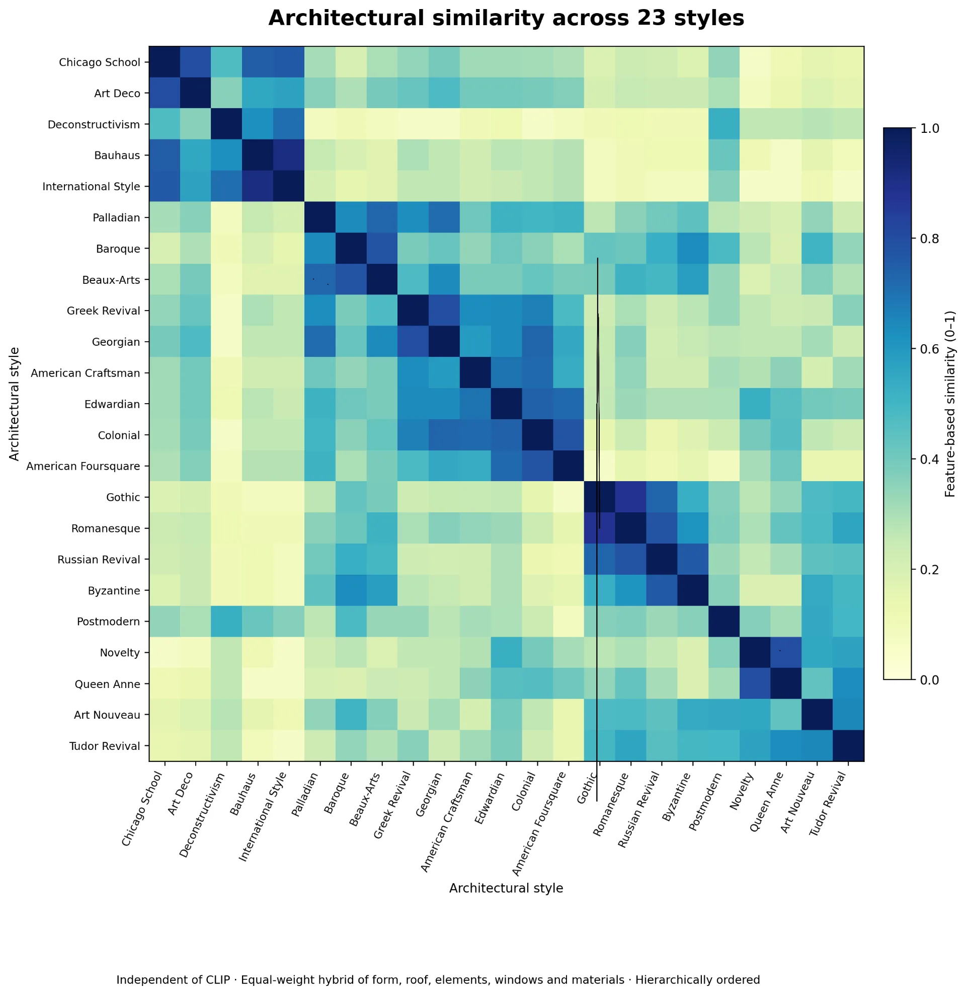
Every entry represents the architectural similarity between two types:

Equation 14.

The matrix is symmetric: the similarity between Gothic and Romanesque is identical because the similarity between Romanesque and Gothic.

Every model additionally has most similarity with itself:

Equation 15

Excluding comparisons of a mode with itself, we acquire 253 distinctive pairs of architectural types:

Equation 16.

A few of the strongest relationships recognized by our feature-based measure are proven under in Desk 6.

Architectural Types	Similarity
Bauhaus-Worldwide Model	0.917
Gothic-Romanesque	0.880
Greek Revival-Georgian	0.800
Novelty-Queen Anne	0.800
Chicago College-Artwork Deco	0.800
Colonial-American FourSquare	0.780
Baroque-Beaux Arts	0.780
Russian Revival-Byzantine	0.760

Desk 6.

A number of relationships are per established architectural traits. Bauhaus and Worldwide Model share geometric simplicity and little or no ornamentation. Gothic and Romanesque structure share structural and historic options, whereas Greek Revival and Georgian structure share symmetry and classical proportions.

These examples counsel that our similarity measure produces cheap outcomes. Nevertheless, the scores rely on our alternative of options and their equal weighting. Totally different options or weights might produce completely different outcomes.

5.6 How Related are Architectural Types in Basic?

Earlier than making use of our measure to CLIP’s retrieval outcomes, we examined the distribution of similarity scores throughout all 253 distinct model pairs. The imply architectural similarity was 0.345, and the median was 0.307.

The seventy fifth percentile was 0.460, that means that roughly three-quarters of the model pairs had similarity scores at or under that worth. On the higher finish of the distribution, the ninetieth percentile was 0.639, and the ninety fifth percentile was 0.733. These values set up a reference distribution in opposition to which CLIP’s label mismatches may be evaluated.

A similarity rating of 0.70, for instance, is just not merely a quantity between zero and one. Inside our architectural similarity matrix, it represents a comparatively robust relationship in contrast with most different architectural model pairs.

This permits us to judge a retrieval mismatch in context.

If CLIP retrieves a Romanesque constructing for a Gothic question, we are able to lookup the architectural similarity between these types and decide how that relationship compares with the total distribution. As a substitute of treating each mismatch as equally incorrect, we are able to start distinguishing retrievals involving carefully associated types from these involving considerably completely different architectural traits.

5.7 Two Views on Architectural Similarity

CLIP measures similarity by way of realized picture representations, whereas our feature-based measure compares architectural types. Each have limitations: CLIP could also be influenced by irrelevant visible particulars, and our measure doesn’t evaluate particular person buildings.

However does CLIP retrieve architecturally associated types extra usually than we’d count on by likelihood?

Let’s look at the proof.

6. When CLIP Will get It Flawed, Might It Be Proper?

We now look at whether or not CLIP’s label mismatches replicate significant architectural similarities.

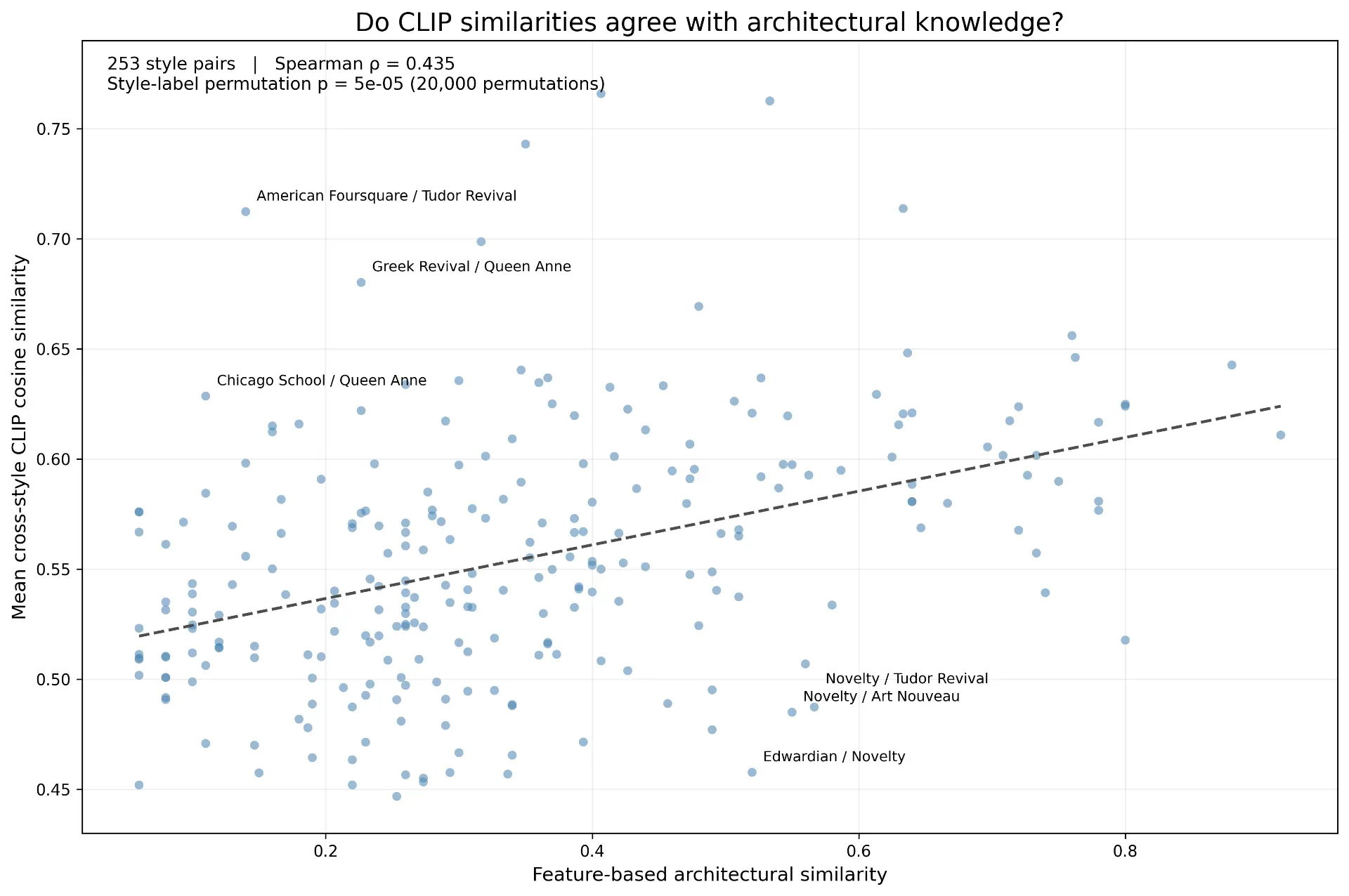
Earlier than analyzing the retrieval outcomes, we in contrast our feature-based similarity scores with the imply CLIP cosine similarity for every of the 253 distinctive architectural model pairs.

The outcomes present a average constructive correlation (Spearman ρ = 0.435). Types with increased feature-based similarity typically obtain increased CLIP similarity scores, though some pairs present substantial disagreement.

6.1 How Architecturally Related Are CLIP’s Mismatches?

We examined CLIP’s 2,465 Precision@1 label mismatches, acquiring the similarity between every question model and its retrieved model from our architectural similarity matrix.

Let qᵢ denote the architectural model of question i, and rᵢ the model of its top-ranked retrieval.

We outline the set of label mismatches as:

Equation 17.

For our dataset, $mathcal=2,465$

For every mismatch, its architectural similarity is:

Equation 18.

the place $M_{textual content{characteristic}}$

The imply architectural similarity amongst mismatches is:

Equation 19.

The distribution offers further perception.

Statistic	Architectural similarity
Imply	0.500
Median	0.473
seventy fifth percentile	0.667
ninetieth percentile	0.800
Most	0.917

Desk 7.

These outcomes point out that a lot of CLIP’s mismatches contain types sharing substantial architectural traits.

Nevertheless, an absolute similarity rating doesn’t inform us how uncommon that resemblance is. A rating of 0.50 is likely to be excessive or low relying on the similarity distribution throughout all architectural types.

To place these outcomes into perspective, we in contrast the architectural similarity of every mismatch with the similarity scores of all 253 distinct architectural model pairs. We then calculated the percentile rank of every mismatch and averaged these ranks. This helps us perceive the place CLIP’s mismatches are inclined to fall inside the general distribution of architectural similarities.

How did we calculate the imply percentile rank of mismatch similarity scores?

We ranked the 253 architectural model pairs in response to their similarity scores. For every of CLIP’s 2,465 mismatches, we decided the place its similarity rating fell inside this distribution.

For instance, a percentile rank of 80 signifies that the mismatch has an architectural similarity rating increased than roughly 80% of all model pairs.

We then calculated the imply percentile rank by including the percentile ranks of all 2,465 mismatches and dividing by 2,465:

Equation 20.

the place P_i is the percentile rank of mismatch i.

What did we discover?

• Imply percentile rank: 71.2. On common, CLIP’s mismatches ranked across the 71st percentile in architectural similarity.

• 51.4% of mismatches fell inside the high 25% of architectural similarities.

• 27.5% fell inside the high 10%.

• 18.6% fell inside the high 5%.

These outcomes present that CLIP’s mismatches have been concentrated amongst architectural types with comparatively excessive similarity scores, relatively than being distributed uniformly throughout all attainable model pairs.

However might this sample come up just because some architectural types happen extra incessantly than others in our dataset?

To reply that query, we carried out a Monte Carlo experiment.

6.2 Are CLIP’s Mismatches Extra Significant Than Likelihood?

A convincing analysis requires greater than displaying that CLIP retrieves architecturally comparable types. We should set up whether or not the noticed similarities exceed what can be anticipated from random retrieval.

Importantly, our dataset doesn’t comprise equal numbers of pictures for each architectural model. A random retrieval is due to this fact extra more likely to return a standard model than a uncommon one. To account for this imbalance, we constructed a frequency-aware random baseline.

For every of the two,465 queries related to a label mismatch, we randomly chosen an alternate architectural model, excluding the question’s personal model. Different types have been sampled proportionally to their frequencies within the dataset. We then calculated the imply architectural similarity between every question model and its randomly chosen various.

This course of was repeated 10,000 occasions, utilizing a set random seed of 42 for reproducibility.

Let $r_i^{(b)}$

The imply similarity for that trial is:

Equation 21.

the place $mathcal=2,465$

We then in contrast the noticed CLIP imply with the distribution of the ten,000 simulated means.

Outcomes

Metric	Worth
Noticed CLIP imply similarity	0.5001
Random baseline imply	0.3500
Random baseline normal deviation	0.0037
95% simulated null interval	0.3429–0.3573
Most simulated imply	0.3638
Monte Carlo trials	10,000
Monte Carlo p-value	0.00009999

The noticed imply architectural similarity of CLIP’s mismatches was roughly 43% increased than the random baseline. Extra importantly, not one of the 10,000 random trials produced a imply similarity as excessive as CLIP’s noticed worth.

This end result offers robust statistical proof that CLIP’s label mismatches exhibit better architectural similarity than can be anticipated from frequency-aware random choice.

We additionally examined whether or not the end result was pushed by a small variety of incessantly confused model pairs. The two,465 mismatches concerned 287 distinct directional model pairs, and the 5 most frequent pairs accounted for less than 11.9% of the mismatches. Thus, the noticed architectural resemblance was not confined to a handful of recurring model confusions.

The conclusion is critical: even when CLIP retrieves a picture with the fallacious architectural label, its alternative is way from random by way of architectural traits.

7. Dialogue: Past Architectural Retrieval

The restrictions of category-based analysis prolong past architectural picture retrieval.

In vogue retrieval, garments from completely different classes could share comparable silhouettes, textures, or design parts. In product search, competing manufacturers could supply practically similar merchandise. In semantic search, paperwork assigned to completely different matters could categorical carefully associated concepts.

These examples illustrate why relevance is determined by the applying. Visible look could matter most in vogue, performance in product search, and that means in doc retrieval.

Enhancing retrieval methods due to this fact requires not solely higher fashions, but in addition analysis strategies that replicate what customers really take into account related.

8. Conclusion

Utilizing 9,315 pictures representing 23 architectural types, we discovered that CLIP’s 2,465 label-mismatched Precision@1 retrievals confirmed considerably better architectural similarity than anticipated below a frequency-aware random baseline, as our Monte Carlo experiment confirmed.

Our findings present that typical categorical analysis can overlook significant relationships captured by embedding-based retrieval methods. They assist complementing Precision@Ok with application-specific similarity measures to offer a extra full evaluation of retrieval high quality.

Thanks for studying!

The dataset used within the article may be discovered at:

https://www.kaggle.com/datasets/dumitrux/architectural-styles-dataset

The whole code for the article may be discovered at:

https://github.com/theomitsa/AI-Architectural-Analysis

Observe: All figures and plots have been created by the creator.

Information license data: CCO: Public area.

https://creativecommons.org/publicdomain/zero/1.0/