Don’t Let Messy Information Bend Your Curves

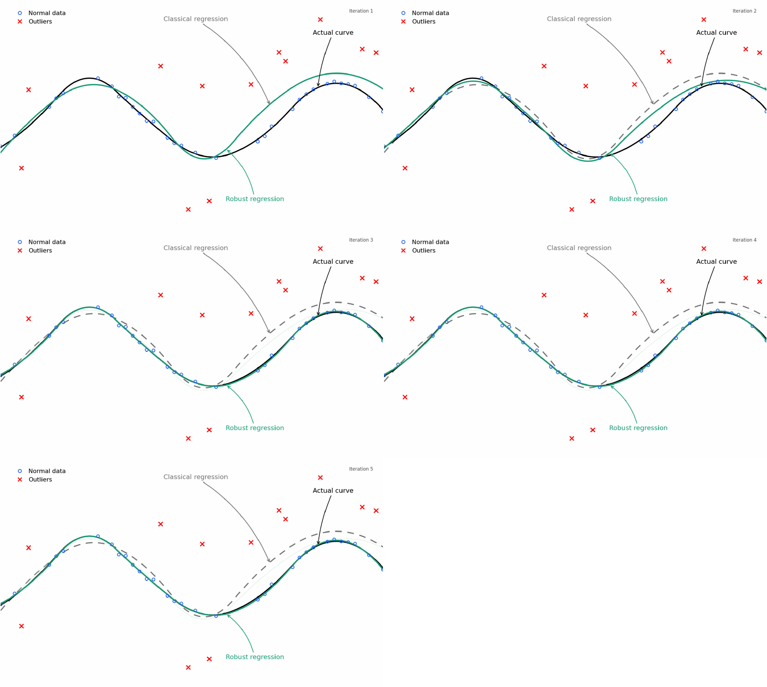
When a Straight Line Stops Being Sufficient

Linear regression earns its recognition for good causes: it’s easy, quick, interpretable, and infrequently surprisingly efficient. However actual relationships don’t all the time cooperate with straight strains.

Some bend progressively. Some flatten. Some change habits throughout completely different areas. Braking distance, crop response, wind-turbine energy, and satellite tv for pc Doppler all present acquainted examples the place curvature is a part of the underlying relationship fairly than a nuisance to be ignored.

The earlier article on this collection saved the mannequin intentionally easy and centered on robustness. I in contrast OLS with Huber regression [1], RANSAC [2], GNC-GM, GNC-TLS [3], and ASOR [4] to see what occurs when contaminated observations attempt to pull a straight-line match away from the nominal relationship.

Now we hold that very same robustness drawback—however give the mannequin extra room to maneuver.

From Straight Strains to Versatile Curves

The pure first step past a line is to introduce polynomial options. Then we encounter a brand new limitation: polynomial flexibility is international, so altering one coefficient can reshape the curve in all places. Splines provide one other route by introducing flexibility regionally.

That offers us two very completely different questions to deal with: which observations ought to the estimator belief, and what shapes ought to the mannequin be able to representing?

The estimator controls belief. The idea controls form.

The primary query is best to see visually. Figures 1 and a couple of present a easy nonlinear instance through which OLS intently follows the underlying relationship when the observations are clear, whereas a sturdy estimator stays a lot nearer to the nominal curve when the info are contaminated.

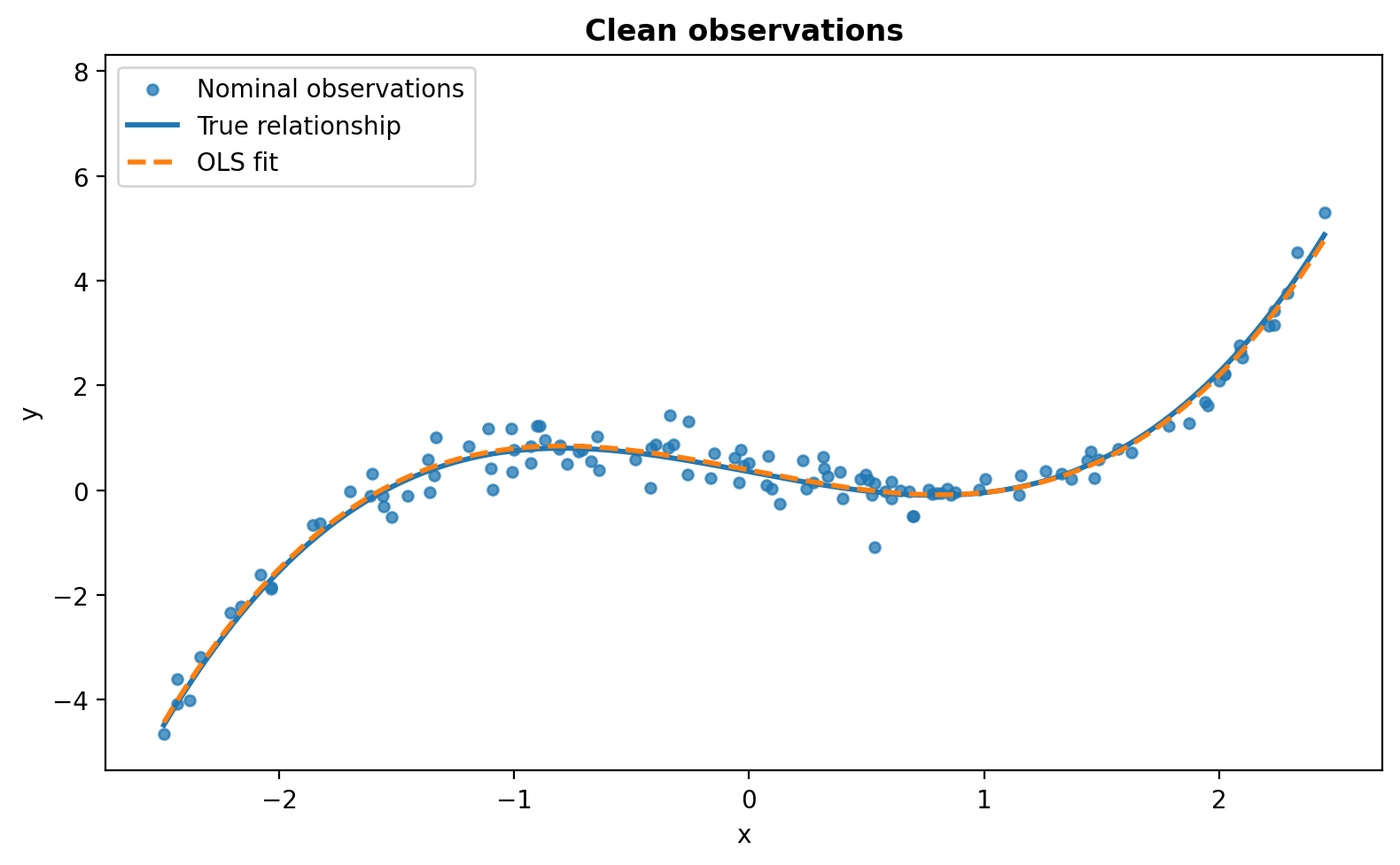
OLS match; polynomial regression

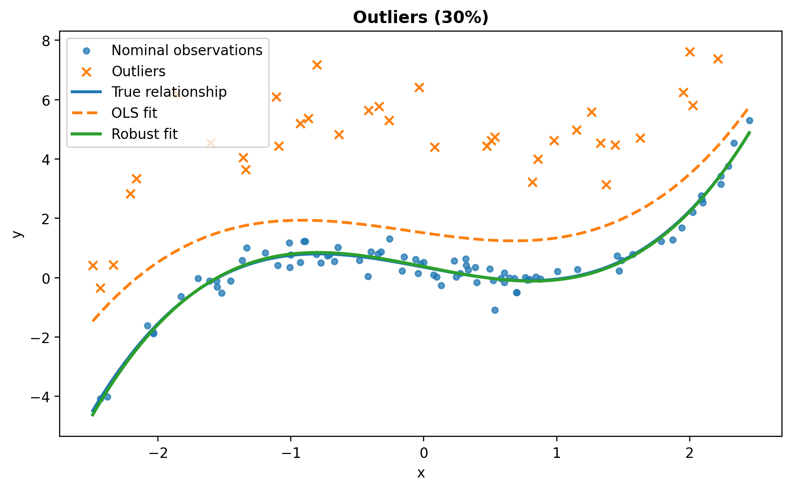
After 30% of the responses are contaminated, the OLS match is pulled away from the underlying nonlinear relationship, whereas the strong match stays a lot nearer to it.

The second query is about illustration: how can we give the mannequin sufficient flexibility to explain a curved relationship? We start with polynomial regression.

Polynomial Regression Via a Linear-Mannequin Lens

Take into account $N$ measurements, the place the $i$-th measurement is modeled as

Right here, the coefficients $β_k$

The measured response $y_i$

Extra typically,

Polynomial regression is due to this fact a linear mannequin in a reworked function house [5].

By stacking the person measurements, the mannequin will be written in matrix type as,

the place, for a quadratic mannequin,

OLS solves

In code, shifting from a line to a polynomial is barely a change within the design matrix:

def polynomial_design(x, diploma):    x = np.asarray(x, dtype=float)    return np.vander(x, N=diploma + 1, rising=True)Phi = polynomial_design(x, diploma=3)beta = np.linalg.lstsq(Phi, y, rcond=None)[0]

For numerical stability, particularly because the polynomial diploma will increase or the $x_i$

Centering shifts the predictor in order that its common is close to zero, whereas scaling divides by a measure of its unfold in order that its values are sometimes of order one. The polynomial phrases are then constructed from this reworked predictor, which retains higher-order powers from changing into excessively giant and improves numerical stability.

The vital level is that nothing elementary has modified. For a line, the $i$-th row of the design matrix is

whereas for a quadratic it turns into

The identical thought extends to higher-order polynomials by including increased powers of $x_i$

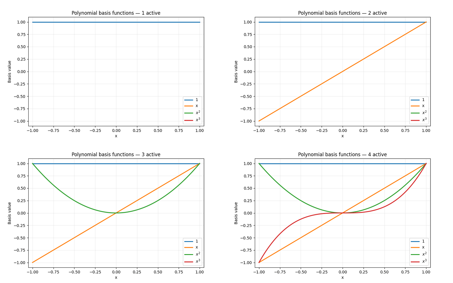
Determine 3 makes this foundation growth seen. Ranging from the fixed and linear phrases, increased powers of the predictor are added to provide the mannequin progressively extra flexibility.

However higher flexibility comes with trade-offs. A level-$p$ polynomial has $p+1$

That international nature is exactly the place splines turn into helpful: they supply flexibility regionally fairly than forcing one polynomial to elucidate every part directly.

When One International Polynomial Is Not Sufficient

Splines introduce flexibility in another way. As an alternative of representing the complete relationship with one international polynomial, they be a part of polynomial items at chosen areas referred to as knots.

B-splines present a handy foundation for developing these piecewise-polynomial curves whereas sustaining clean connections between neighboring items [7].

The spline mannequin will be written as

the place $B_{j,p}(x)$

How the B-Spline Foundation Is Fashioned

A B-spline foundation is decided by the spline diploma and the knot areas.

Suppose the noticed vary is $[a,b]$ the spline diploma is $p$ and we select $Ok$ inside knots $kappa_1,kappa_2,ldots,kappa_K$

The variety of ensuing foundation capabilities is $M=Ok+p+1$

These foundation capabilities are constructed from the knot vector utilizing the Cox–de Boor recursion [7]. The recursion begins with the degree-zero foundation capabilities,

Right here, $t_j$

For the quadratic spline used right here,

the place a time period is taken as zero each time its denominator is zero.

The idea is due to this fact constructed progressively as

The degree-zero capabilities are piecewise fixed, the degree-one capabilities are piecewise linear, and the ultimate $B_{j,2}(x)$

Determine 4 visualizes this recursive development. The lower-degree capabilities are intermediate steps used to generate the ultimate quadratic B-spline foundation capabilities.

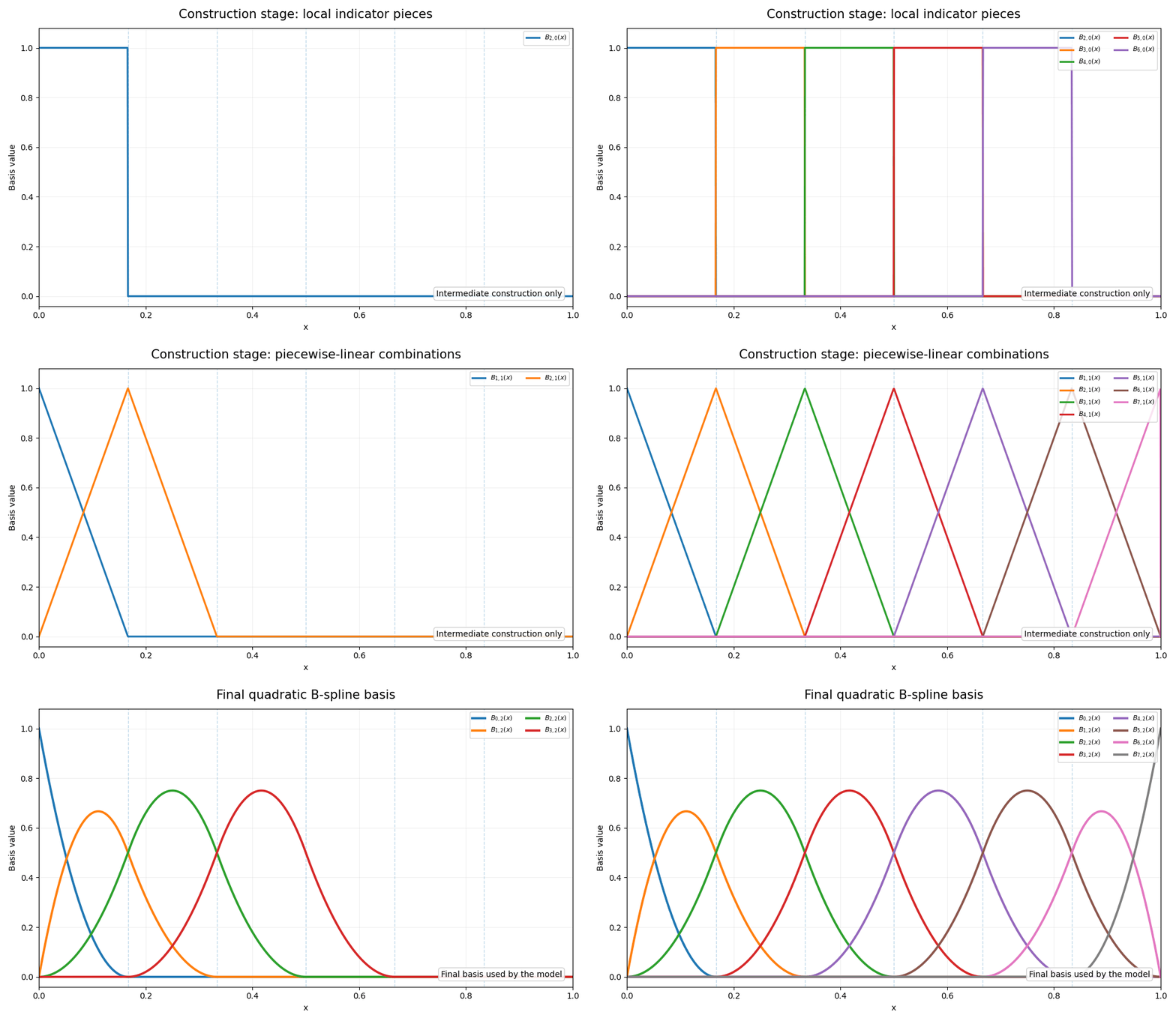
In contrast to the powers utilized in a worldwide polynomial, every quadratic B-spline foundation operate has native assist,

Every coefficient due to this fact influences solely a restricted area of the fitted curve. With easy inside knots, the neighboring quadratic items additionally be a part of with a steady first by-product [7].

As soon as the idea capabilities are fashioned, the $i$-th commentary is represented by

Stacking these rows provides the acquainted regression mannequin,

Polynomial and spline regression due to this fact differ in how $boldsymbol{Phi}$ is constructed, however each stay linear within the unknown coefficients as soon as the idea is fastened.

With the illustration drawback in place, we are able to now return to the primary query: which observations ought to the estimator belief?

Not All Dangerous Information Is the Similar

When Measurements Are Lacking

Measurements can go lacking due to dropouts, failed recordings, or skipped readings. Lacking values could also be eliminated, imputed, or dealt with by way of probabilistic strategies corresponding to Expectation–Maximization [6]. Right here, we intentionally use the only choice—prefiltering measurements containing non-finite values—as a result of our curiosity lies within the impact of outliers on curve becoming. This shouldn’t be interpreted as a normal suggestion for dealing with lacking observations.

legitimate = np.isfinite(Phi).all(axis=1) & np.isfinite(y)Phi = Phi[valid]y = y[valid]

As soon as the explicitly lacking measurements have been dealt with, a tougher drawback stays: what ought to we do with observations which can be current however unreliable?

The Outlier Drawback

Outliers can seem due to defective readings, interference, or uncommon working situations. In contrast to lacking values, they’re current and finite, and should initially look completely authentic.

This creates a chicken-and-egg drawback: we’d like a dependable mannequin to find out which observations are inconsistent with the underlying relationship, however those self same observations can distort the mannequin used to determine them.

Sturdy estimators deal with this drawback by limiting the affect of observations which can be inconsistent with the fitted relationship.

The Similar Six Estimators, a Completely different Foundation

Altering the idea doesn’t require us to revamp the strong estimator.

Huber regression reduces the affect of enormous residuals [1]. RANSAC searches for a consensus among the many observations [2]. GNC-GM and GNC-TLS progressively remodel simpler optimization issues into extra aggressive strong aims [3]. ASOR adaptively estimates how strongly every commentary ought to contribute to the match [4].

For weighting-based strong estimators, the regression step can nonetheless be written as

What adjustments is the idea used to assemble the function vector.

For a cubic polynomial,

whereas for an eight-function spline,

The idea determines what shapes the mannequin can signify. The strong estimator determines how a lot every commentary is trusted.

If the identical estimators can be utilized with completely different bases, the subsequent query is whether or not they nonetheless behave the identical manner because the mannequin turns into extra versatile.

Stress-Testing

To reply that query, we repeat the identical household of robustness experiments for curved fashions.

We take into account three mannequin courses,

and apply the identical six estimators,

The benchmark covers a number of types of contamination: zero-mean Gaussian alternative outliers, biased Gaussian alternative outliers, biased uniform alternative outliers, and observations generated from a coherent competing relationship. We additionally range the contamination ratio from $0$ to $90$, the variety of measurements, the nominal noise stage, and report the computational value. Every precise situation is repeated over 30 Monte Carlo realizations. The entire simulation pocket book, full Monte Carlo outcomes, and figures can be found within the GitHub repository.

Prediction error is measured in opposition to the true noiseless relationship on a dense analysis grid:

For the nominal-noise sweep, we additionally report

To isolate the impact of mannequin richness from the impact of adjusting the underlying curve, we additionally carry out a managed experiment through which the identical quadratic relationship and the identical contaminated observations are fitted utilizing all three bases. The fashions then use 3, 4, and eight coefficients, respectively, whereas making an attempt to get better precisely the identical floor fact.

The fascinating query isn’t merely whether or not strong estimation nonetheless works with curves, however what adjustments because the illustration turns into richer.

Does estimator rating change because the variety of coefficients will increase? How does RANSAC behave as its minimal pattern grows? Do richer fashions require extra knowledge earlier than their efficiency stabilizes? Does native spline assist change how contamination deforms the fitted curve? And does computational value change sufficient to change the sensible trade-offs?

What the Stress Exams Reveal

The managed experiment provides the clearest view of what adjustments because the illustration turns into richer. In every Monte Carlo realization, all three representations are fitted to the identical $N=100$

At $30$ biased Gaussian contamination, GNC-TLS produces median NRMSE values of $0.246$, $0.276$and $0.485$ for the quadratic, cubic, and spline representations. ASOR follows an analogous sample, with of $0.257$, $0.307$and $0.469$. The transfer from three to 4 coefficients due to this fact causes solely a modest loss. The eight-function spline is noticeably extra demanding.

RANSAC reacts rather more strongly. Underneath the identical knowledge and contamination stage, its median NRMSE rises from $0.273$ for the quadratic match to $0.383$ for the cubic and $1.384$ for the spline.

The impact is seen even with out contamination: RANSAC’s median NRMSE will increase from $0.179$ for the quadratic mannequin to $0.625$ for the spline.

A richer foundation can signify extra shapes, however it additionally provides the estimator extra parameters to get better.

RANSAC is especially delicate as a result of its minimal pattern grows with the variety of coefficients.

For the three fashions thought of right here,

If the inlier fraction is $w$, the variety of hypotheses wanted to acquire an all-inlier minimal pattern with confidence $p$ is

At $50$ contamination and $p=0.999$

The runtime outcomes inform the identical story. At $50$ biased Gaussian contamination, median RANSAC runtime will increase from about $2.1$ms for the quadratic mannequin to $3.4$ms for the cubic and $17.4$ms for the spline.

The algorithm itself has not modified. The mannequin it should hypothesize has.

Richer Fashions Want Extra Information

The sample-size sweep exhibits the opposite facet of the trade-off. Underneath $50$ biased Gaussian contamination, the spline turns into rather more secure as extra measurements can be found.

For the spline, GNC-TLS NRMSE falls from $1.641$ at $N=50$

OLS behaves in another way. Its error stays excessive even because the variety of measurements grows, as a result of further knowledge scale back variability however don’t take away the systematic pull created by the contamination.

So the lesson isn’t that splines are inherently much less strong.

Versatile fashions want sufficient reliable knowledge to assist the additional levels of freedom.

The Contamination Sample Nonetheless Issues

There isn’t a common estimator rating.

Underneath biased contamination, GNC-TLS and ASOR typically present the bottom prediction errors by way of average contamination, with GNC-GM typically shut behind.

When the alternative errors are zero imply, nevertheless, the variations turn into a lot smaller. For the spline at $50$ zero-mean Gaussian contamination, the median NRMSE values are $0.526$ for Huber, $0.540$ for GNC-GM, $0.554$ for ASOR, and $0.579$ for GNC-TLS.

On this benchmark, zero-mean alternative errors are typically much less damaging than equally scaled biased errors as a result of they don’t constantly push the slot in one path.

The nominal-noise sweep provides one other helpful verify. After normalizing by $sigma_{mathrm{in}}$

Native Help Comprises Distortion; It Does Not Take away It

Splines introduce an impact that international polynomials would not have: native assist.

In an illustrative experiment, we contaminate solely a part of the observations inside a slender area whereas leaving the remaining native measurements nominal.

With OLS, the cubic polynomial provides an RMSE of about $22.6$ contained in the contaminated area and $13.6$ exterior it. The spline is distorted extra strongly contained in the contaminated area, with an RMSE of $40.9$, however barely much less exterior it, at $12.1$.

This is a crucial distinction.

Native assist can confine deformation to a smaller area, however it doesn’t make contaminated observations innocent.

As soon as strong weighting is launched, the distortion drops considerably for each representations. On this instance, ASOR reduces the native and nonlocal errors to roughly $7.0$ and $4.8$ for the cubic mannequin, and $12.6$ and $5.5$ for the spline.

The 2 mechanisms due to this fact remedy completely different issues:

Native assist controls the place mannequin flexibility acts. Sturdy estimation controls how strongly unreliable observations act.

When the Outliers Kind One other Curve

Random alternative outliers are tough, however a coherent competing relationship creates a unique drawback.

At low and average contamination, the strong estimators can nonetheless get better the nominal curve. As the 2 buildings strategy equal illustration, nevertheless, the issue turns into ambiguous and completely different Monte Carlo realizations might favor completely different relationships.

As soon as the competing curve turns into the bulk construction, the strong estimators typically observe it.

This isn’t merely an optimization failure. A single-model estimator has no approach to know which of two internally constant relationships is the bodily right one with out further data.

Sturdy estimation can suppress observations that disagree with the dominant mannequin.

It can’t determine which of two coherent fashions must be trusted.

Taken collectively, these experiments present that altering the idea impacts greater than the shapes a mannequin can signify. It additionally adjustments how a lot knowledge the estimator wants, how costly consensus-based strategies turn into, and the way contamination propagates throughout the fitted curve.

The managed experiments isolate these results. We now flip to application-inspired examples the place robustness and mannequin flexibility turn into separate sensible necessities.

Case Examine 1: Wind-Turbine Energy Curves

Robustness isn’t the identical as mannequin flexibility.

Wind-turbine energy curves describe the anticipated relationship between wind pace and generated energy. Dependable estimation of this relationship is helpful for efficiency monitoring and for figuring out working situations that deviate from regular turbine habits.

In apply, SCADA data might comprise low-power or in any other case irregular observations attributable to curtailment, faults, shutdowns, or measurement points [8]. These observations can distort the estimated nominal energy curve, making this a pure utility for strong regression.

The wind-turbine instance is especially helpful as a result of it separates two issues which can be typically confused:

Can the estimator resist irregular observations?

and

Can the chosen mannequin signify the underlying relationship?

To make this distinction clear, we first assemble a area through which polynomial regression is the right mannequin. We then lengthen the area till a single international polynomial turns into solely an approximation.

First Isolate the Robustness Drawback

For this artificial instance, let the rated pace be $12,textual content{m/s}$.

Under rated pace, outline

and

As a result of $t$ is linear in $v$, this expression is precisely a cubic polynomial in wind pace.

If we match a cubic polynomial over this area, the mannequin household is accurately specified. The experiment due to this fact isolates the impact of contamination.

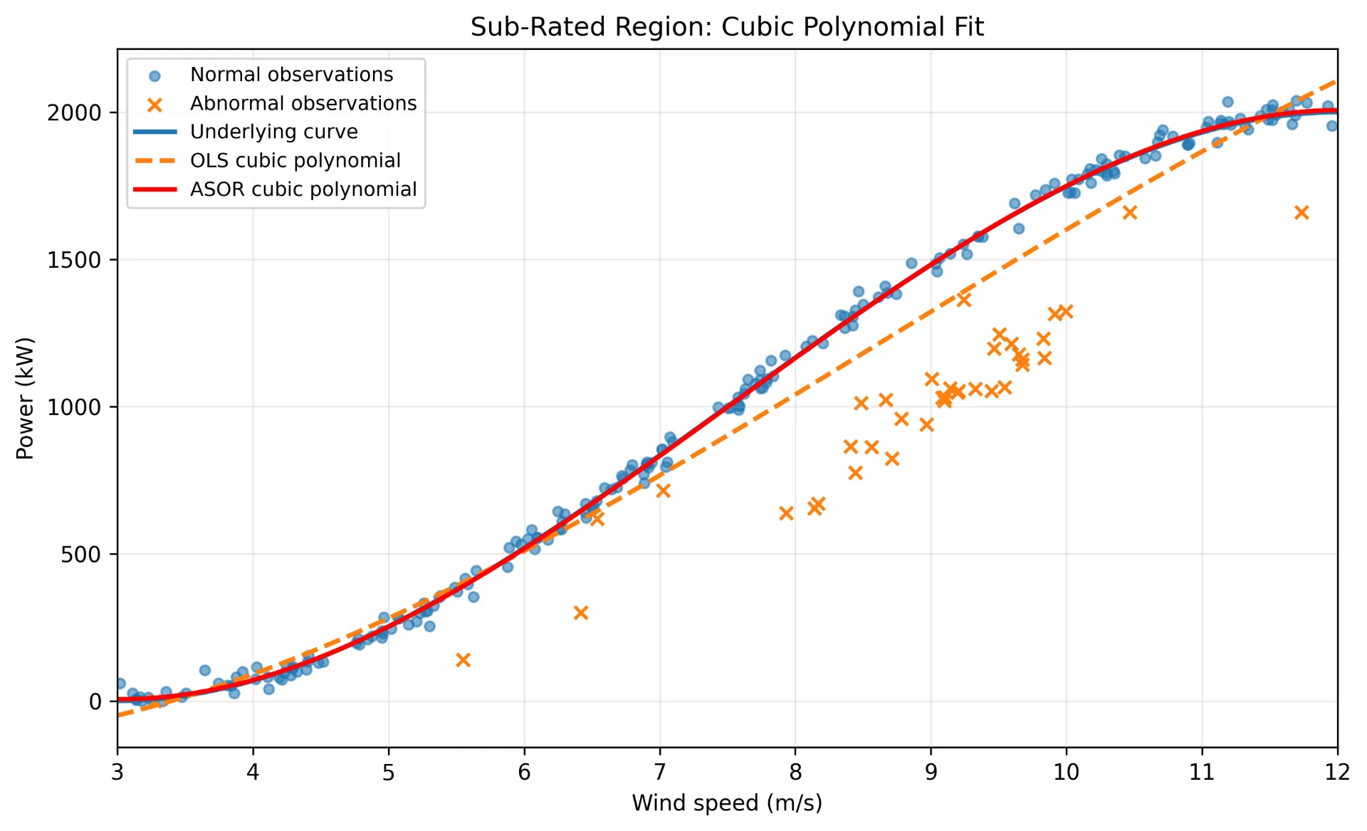
For this realization, the prediction RMSE is roughly $91.4,textual content{kW}$ for OLS and $2.7,textual content{kW}$ for ASOR.

Right here the interpretation is easy:

The mannequin was applicable. The estimator was the issue.

Sturdy estimation addresses the contamination drawback with out requiring us to alter the mannequin household.

Then Expose the Illustration Drawback

Now lengthen the identical floor fact past rated pace:

The connection is now piecewise outlined:

One international polynomial is now not the true mannequin.

No nonconstant finite-degree polynomial can precisely reproduce this form. If a polynomial $q(v)$ satisfies $q(v)=2000$

A world polynomial can due to this fact solely approximate the curved-to-flat relationship.

The issue has modified. We’re now not asking solely whether or not the estimator is strong; we should additionally ask whether or not the chosen foundation can signify the underlying relationship.

Can a Greater-Order Polynomial Resolve the Drawback?

One apparent response is to extend the polynomial diploma.

A fourth-order polynomial makes use of

This supplies extra flexibility than a cubic, and with strong estimation it performs moderately nicely.

Nevertheless, all 5 polynomial foundation capabilities stay international. The identical coefficients should concurrently describe the low-speed rise, the steep center area, the transition close to rated pace, and the high-speed plateau.

A spline provides flexibility in another way. As an alternative of introducing more and more excessive international powers, it makes use of regionally supported foundation capabilities that may adapt to completely different elements of the curve.

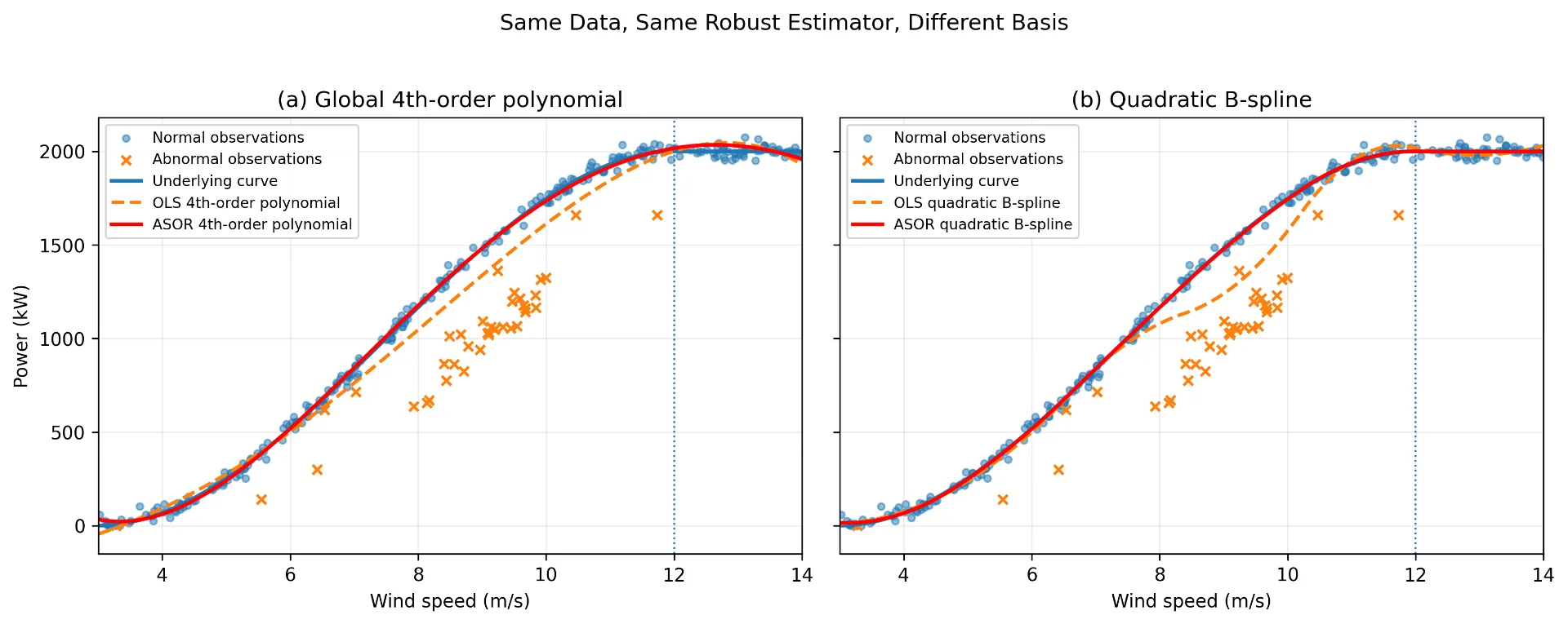
For a similar illustrative realization, over the complete $3–14,textual content{m/s}$ interval, the ASOR fourth-order polynomial provides an RMSE of roughly $14.5,textual content{kW}$, in contrast with $4.2,textual content{kW}$ for the ASOR quadratic B-spline.

That distinction is vital:

Sturdy estimation can cease irregular observations from bending an excellent mannequin. It can’t flip the improper foundation into the proper one.

On this instance, ASOR addresses the contamination, whereas the spline addresses the illustration.

Case Examine 2: Predicting The place GNSS Doppler Goes Subsequent

GNSS Doppler evolves easily with satellite tv for pc–receiver movement. Brief-term prediction may also help bridge transient measurement gaps and supply an anticipated Doppler pattern in opposition to which irregular measurements related to interference or monitoring disturbances will be in contrast.

This makes Doppler prediction a helpful robust-regression instance: corrupted measurements can distort the fitted pattern and, consequently, the expected Doppler.

Over a brief commentary window, we use a low-order polynomial as a compact native approximation to the Doppler trajectory.

The workflow is

The instance accommodates each lacking and corrupted measurements. Lacking samples are excluded in line with the preprocessing assumption launched earlier, whereas corrupted samples stay within the knowledge and have to be dealt with by the estimator.

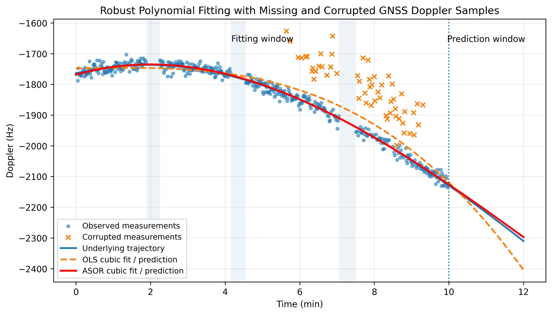
OLS tries to elucidate the corrupted measurements, inflicting the fitted polynomial to bend towards the corrupted cluster. ASOR reduces their affect and preserves a trajectory that continues to be a lot nearer to the nominal Doppler evolution.

This turns into notably vital when the fitted curve is extrapolated past the commentary window. A average becoming error contained in the noticed area can develop considerably when the polynomial is projected into the long run.

On this artificial illustration, the short-horizon prediction RMSE is roughly $46.4,textual content{Hz}$ for OLS and $7.9,textual content{Hz}$ for ASOR.

The declare right here is intentionally native. A satellite tv for pc Doppler trajectory isn’t assumed to observe one cubic polynomial indefinitely. As an alternative, a low-order polynomial supplies a compact approximation over a brief commentary window.

This results in one other vital lesson:

Interpolation and extrapolation will not be the identical drawback.

Sturdy becoming can enhance each, however extrapolation stays inherently extra delicate as a result of future factors are now not surrounded by noticed knowledge.

What Survives When the Line Turns into a Curve?

Essentially the most helpful lesson from all of those examples isn’t tied to at least one polynomial diploma or one explicit spline.

It’s the foundation view.

A straight line makes use of

A polynomial makes use of

A spline replaces international powers with regionally supported capabilities,

As soon as the idea is fastened, all of those fashions return to the identical type:

That’s the reason the strong estimators switch so naturally.

The sensible workflow is due to this fact simple:

1. Select a foundation that may signify the connection of curiosity.

2. Middle and scale predictors when polynomial powers turn into poorly conditioned.

3. Take away identifiable lacking rows earlier than becoming when complete-case evaluation is suitable.

4. Use strong estimation when finite observations should still be contaminated.

5. Use sufficient observations to assist the chosen foundation.

6. Deal with extrapolation extra cautiously than interpolation.

A richer foundation makes the mannequin extra expressive, however it doesn’t make unreliable observations reliable. Sturdy estimation makes the match much less delicate to contamination, however it can’t rescue an inappropriate mannequin.

These are two completely different issues.

Subsequent within the collection. We transfer past polynomials and splines to richer representations for capturing advanced nonlinear and periodic construction.

References

[1] P. J. Huber, “Sturdy Estimation of a Location Parameter,” The Annals of Mathematical Statistics, vol. 35, no. 1, pp. 73–101, 1964.

[2] M. A. Fischler and R. C. Bolles, “Random Pattern Consensus: A Paradigm for Mannequin Becoming with Functions to Picture Evaluation and Automated Cartography,” Communications of the ACM, vol. 24, no. 6, pp. 381–395, 1981.

[3] H. Yang, P. Antonante, V. Tzoumas, and L. Carlone, “Graduated Non-Convexity for Sturdy Spatial Notion: From Non-Minimal Solvers to International Outlier Rejection,” IEEE Robotics and Automation Letters, vol. 5, no. 2, pp. 1127–1134, 2020.

[4] A. H. Chughtai, M. Tahir, and M. Uppal, “Bayesian Heuristics for Sturdy Spatial Notion,” IEEE Transactions on Instrumentation and Measurement, vol. 73, pp. 1–11, 2024.

[5] T. Hastie, R. Tibshirani, and J. Friedman, The Components of Statistical Studying: Information Mining, Inference, and Prediction, 2nd ed., Springer, 2009.

[6] R. J. A. Little and D. B. Rubin, Statistical Evaluation with Lacking Information, third ed., Wiley, 2019.

[7] C. de Boor, A Sensible Information to Splines, revised ed., Springer, 2001.

[8] Y. Wang, D. G. Infield, B. Stephen, and S. J. Galloway, “Copula-Primarily based Mannequin for Wind Turbine Energy Curve Outlier Rejection,” Wind Vitality, vol. 17, no. 11, pp. 1677–1688, 2014.

Get in contact 👋

For extra of my work, discover my GitHub, or join with me on LinkedIn. I welcome questions, new concepts, and alternatives to collaborate in Information science, AI and Statistical Sign Processing. If you happen to get pleasure from my articles, sharing them with others helps these conversations attain extra individuals.

All data-driven figures have been generated through simulations by the creator. The featured picture was created with the help of AI.