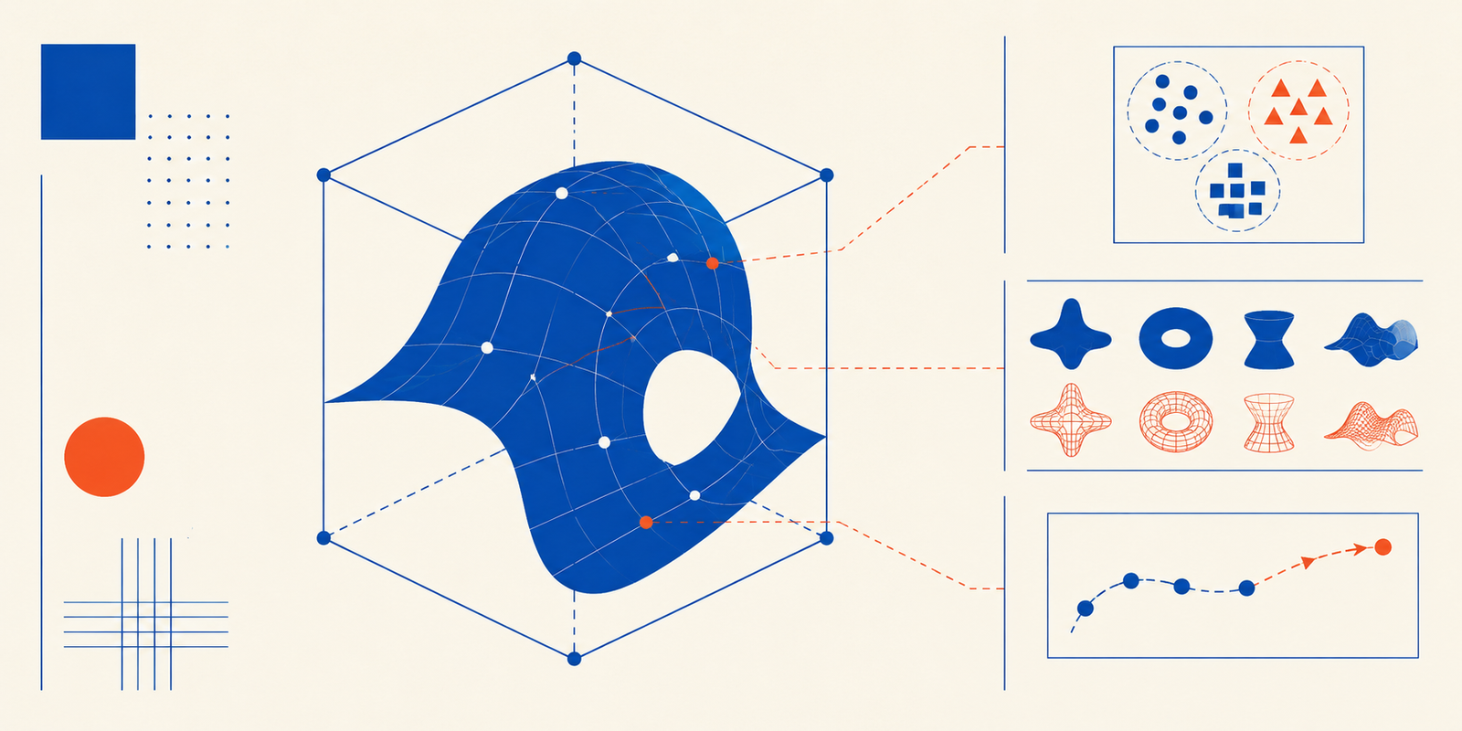
On this article, you’ll study what latent areas are and the way they serve three distinct roles — descriptive, generative, and predictive — throughout a variety of machine studying purposes.
Matters we’ll cowl embody:
- How latent areas compress high-dimensional knowledge into structured numerical representations utilizing methods like Principal Part Evaluation.
- How the generative function of latent areas allows the creation of totally new knowledge factors by means of interpolation.
- How the predictive function of latent areas powers similarity-based purposes corresponding to recommender programs and RAG pipelines.
Introduction
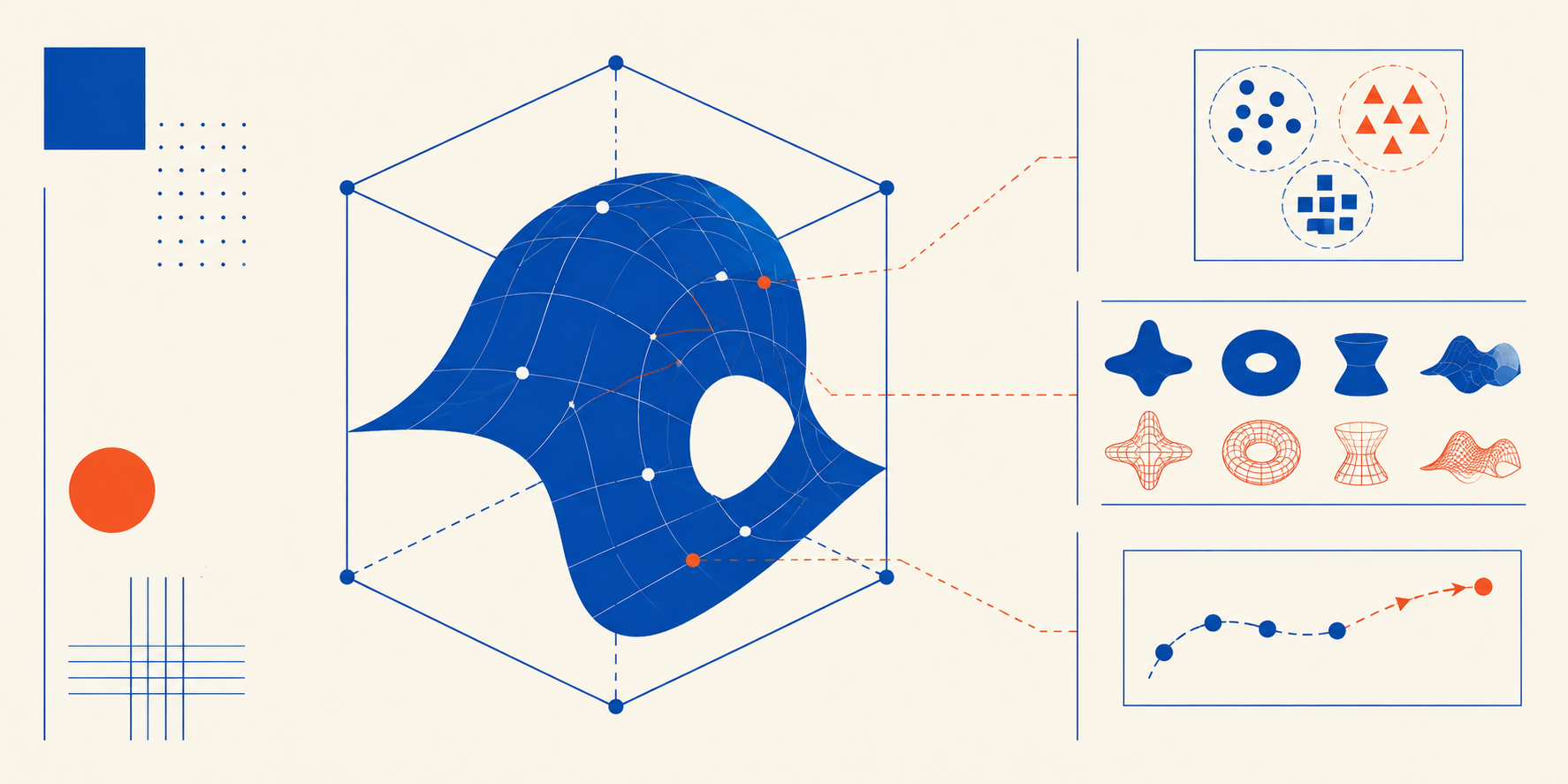
Consider a “secret”, multi-dimensional map through which machine studying fashions treasure the “essence” of complicated, real-world knowledge. That’s the first function of latent areas: compressed, numerical knowledge representations containing the summary options and hidden relationships of the unique, uncooked knowledge they arrive from — be it uncooked picture pixels, audio, textual content, or just high-dimensional, structured knowledge like buyer conduct historical past.
This text analyzes, illustrates, and categorizes the core capabilities and function of latent areas in machine studying fashions. Particularly, we distinguish between three roles: descriptive, generative, and predictive. Let’s unveil how latent areas work beneath every of those hats by means of some concise, runnable code examples you’ll be able to simply take a look at in a Python pocket book.
1. The Descriptive Function: Structuring and Representing Knowledge
Advanced knowledge usually must be summarized and structured in a extra digestible kind earlier than feeding it to downstream machine studying fashions, extracting significant data into related options and discarding irrelevant or redundant ones. That’s the aim of the descriptive function in latent areas: a characteristic extractor compresses high-dimensional inputs into key traits, encoding them numerically. For instance, in a dataset of uncooked, high-quality portrait photographs, disentangling elements like the topic’s pose or lighting retains background noise apart whereas the core semantic data is preserved.
One specific approach that’s extensively used to compress high-dimensional knowledge right into a lower-dimensional area (a smaller variety of options, in easier phrases) is Principal Part Evaluation, or PCA for brief. Whereas PCA doesn’t extract tangible options like lighting or pose, it’s nonetheless a very fashionable approach to drastically compress the unique knowledge options (based mostly on algebraic projections) whereas minimizing the lack of necessary data describing the unique knowledge — this necessary data underlying the unique knowledge is usually often known as variance within the context of PCA and dimensionality discount methods as a complete.
This instance reveals tips on how to apply PCA to compress 3D knowledge right into a 2D latent area that maintains the unique 3D knowledge’s descriptive properties and relationships as a lot as attainable:
|
from sklearn.decomposition import PCA import numpy as np
# Uncooked high-dimensional knowledge: 3 gadgets, 3 options per merchandise raw_data = np.array([[1.1, 2.2, 3.3], [1.0, 2.1, 3.1], [8.1, 9.2, 9.9]])
# Compressing right into a 2D Latent Area map pca = PCA(n_components=2) latent_space_map = pca.fit_transform(raw_data)
print(“Descriptive Latent Area (Compressed Knowledge):n”, latent_space_map) |
Output:
|
Descriptive Latent Area (Compressed Knowledge): [[–3.88962445e+00 4.39634517e–02] [–4.11856576e+00 –4.31334646e–02] [ 8.00819021e+00 –8.29987064e–04]] |
The instance is very simple for example the idea, however in observe, you would possibly apply PCA to compress hundreds of options into, say, a pair hundred at most.
2. The Generative Function: Creating New Knowledge
Acquiring latent area representations from knowledge will also be leveraged as a canvas for creating fully new knowledge cases. The generative function consists of making new knowledge factors by randomly sampling characteristic values that “make sense” for such factors, or by interpolating between present ones. The important thing side to understand right here is: which values make sense for each characteristic — in different phrases, how do the values in every latent area characteristic distribute? Consider it, in its easiest kind, as taking a mathematical stroll between two completely different present factors and mixing their respective characteristic values in infinitely some ways to create entire new outputs: new factors, corresponding to photographs.
That is the core concept behind trendy AI picture turbines, voice synthesizers, and so forth. These programs depend on generative deep studying fashions like autoencoders, adversarial fashions, and even transformers. Whereas these are remarkably complicated and complex fashions, their core concepts are based mostly on interpolating factors in a latent area, as proven within the code under:
|
# Deciding on two distinct factors in our latent area map point_a = latent_space_map[0] point_b = latent_space_map[2]
# Interpolation: Producing a brand new latent level midway between them generated_latent_point = 0.5 * point_a + 0.5 * level_b
# Decoding the brand new level again into the unique 3D uncooked knowledge area generated_raw_data = pca.inverse_transform(generated_latent_point)
print(“Newly Generated Knowledge Level:n”, generated_raw_data) |
Output:
|
Newly Generated Knowledge Level: [4.6 5.7 6.6] |
Take this mathematical idea to the acute, and also you get one thing like an AI that may modify an individual’s eye colour in a supplied picture to make it darker or brighter, for example.
3. The Predictive Function: Similarity and Forecasting
How does the AI behind recommender engines guess what video you need to watch subsequent? Or how does it effectively and reliably determine your facial traits by means of the immigration gates on arrival at a vacation spot airport after a long-haul flight? Latent areas enter the scene once more. The story is partly acquainted: high-dimensional, complicated knowledge like consumer conduct historical past or high-resolution photographs are compressed right into a latent illustration for extra environment friendly and efficient administration whereas retaining key traits. On high of that, the predictive function makes use of latent area coordinates to calculate similarities amongst knowledge factors, draw determination boundaries, and forecast outcomes like essentially the most possible subsequent video to observe or the closest-matching face to the one in entrance of the safety digicam.
In a video recommender system, for instance, movies clustered close to one another share key traits, making it simpler to categorise them, segregate them into classes, or gas correct, related suggestions.
This instance code reveals tips on how to use cosine similarity to foretell essentially the most intently associated knowledge level to a brand new consumer enter:
|
from sklearn.metrics.pairwise import cosine_similarity
# A brand new, unknown merchandise mapped into the latent area new_item_latent = np.array([[0.0, 1.0]])
# Measuring similarity between the brand new merchandise and our present latent map similarity_scores = cosine_similarity(new_item_latent, latent_space_map)
# Greater rating equals nearer geometric relationship in latent area print(“Predictive Similarity Scores:n”, similarity_scores) |
Output:
|
Predictive Similarity Scores: [[ 0.01130203 –0.01047236 –0.00010364]] |
This similarity-based and predictive precept can also be leveraged in trendy LLM-based purposes like RAG programs, through which a consumer question is translated right into a numerical latent illustration known as an embedding, and its similarity to present doc embeddings in a big database is calculated to retrieve essentially the most semantically related texts to the unique question.
Wrapping Up
Whether or not you intention to explain the principle traits of a dataset, generate novel artwork, or predict the subsequent favourite video to observe, latent areas are a helpful, foundational idea all through the machine studying panorama. Mapping messy, real-world knowledge into structured numerical representations is the grasp recipe for compressing, constructing, and connecting concepts throughout all kinds of purposes.
On this article, you’ll study what latent areas are and the way they serve three distinct roles — descriptive, generative, and predictive — throughout a variety of machine studying purposes.
Matters we’ll cowl embody:
- How latent areas compress high-dimensional knowledge into structured numerical representations utilizing methods like Principal Part Evaluation.
- How the generative function of latent areas allows the creation of totally new knowledge factors by means of interpolation.
- How the predictive function of latent areas powers similarity-based purposes corresponding to recommender programs and RAG pipelines.
Introduction
Consider a “secret”, multi-dimensional map through which machine studying fashions treasure the “essence” of complicated, real-world knowledge. That’s the first function of latent areas: compressed, numerical knowledge representations containing the summary options and hidden relationships of the unique, uncooked knowledge they arrive from — be it uncooked picture pixels, audio, textual content, or just high-dimensional, structured knowledge like buyer conduct historical past.
This text analyzes, illustrates, and categorizes the core capabilities and function of latent areas in machine studying fashions. Particularly, we distinguish between three roles: descriptive, generative, and predictive. Let’s unveil how latent areas work beneath every of those hats by means of some concise, runnable code examples you’ll be able to simply take a look at in a Python pocket book.
1. The Descriptive Function: Structuring and Representing Knowledge
Advanced knowledge usually must be summarized and structured in a extra digestible kind earlier than feeding it to downstream machine studying fashions, extracting significant data into related options and discarding irrelevant or redundant ones. That’s the aim of the descriptive function in latent areas: a characteristic extractor compresses high-dimensional inputs into key traits, encoding them numerically. For instance, in a dataset of uncooked, high-quality portrait photographs, disentangling elements like the topic’s pose or lighting retains background noise apart whereas the core semantic data is preserved.
One specific approach that’s extensively used to compress high-dimensional knowledge right into a lower-dimensional area (a smaller variety of options, in easier phrases) is Principal Part Evaluation, or PCA for brief. Whereas PCA doesn’t extract tangible options like lighting or pose, it’s nonetheless a very fashionable approach to drastically compress the unique knowledge options (based mostly on algebraic projections) whereas minimizing the lack of necessary data describing the unique knowledge — this necessary data underlying the unique knowledge is usually often known as variance within the context of PCA and dimensionality discount methods as a complete.
This instance reveals tips on how to apply PCA to compress 3D knowledge right into a 2D latent area that maintains the unique 3D knowledge’s descriptive properties and relationships as a lot as attainable:
|
from sklearn.decomposition import PCA import numpy as np
# Uncooked high-dimensional knowledge: 3 gadgets, 3 options per merchandise raw_data = np.array([[1.1, 2.2, 3.3], [1.0, 2.1, 3.1], [8.1, 9.2, 9.9]])
# Compressing right into a 2D Latent Area map pca = PCA(n_components=2) latent_space_map = pca.fit_transform(raw_data)
print(“Descriptive Latent Area (Compressed Knowledge):n”, latent_space_map) |
Output:
|
Descriptive Latent Area (Compressed Knowledge): [[–3.88962445e+00 4.39634517e–02] [–4.11856576e+00 –4.31334646e–02] [ 8.00819021e+00 –8.29987064e–04]] |
The instance is very simple for example the idea, however in observe, you would possibly apply PCA to compress hundreds of options into, say, a pair hundred at most.
2. The Generative Function: Creating New Knowledge
Acquiring latent area representations from knowledge will also be leveraged as a canvas for creating fully new knowledge cases. The generative function consists of making new knowledge factors by randomly sampling characteristic values that “make sense” for such factors, or by interpolating between present ones. The important thing side to understand right here is: which values make sense for each characteristic — in different phrases, how do the values in every latent area characteristic distribute? Consider it, in its easiest kind, as taking a mathematical stroll between two completely different present factors and mixing their respective characteristic values in infinitely some ways to create entire new outputs: new factors, corresponding to photographs.
That is the core concept behind trendy AI picture turbines, voice synthesizers, and so forth. These programs depend on generative deep studying fashions like autoencoders, adversarial fashions, and even transformers. Whereas these are remarkably complicated and complex fashions, their core concepts are based mostly on interpolating factors in a latent area, as proven within the code under:
|
# Deciding on two distinct factors in our latent area map point_a = latent_space_map[0] point_b = latent_space_map[2]
# Interpolation: Producing a brand new latent level midway between them generated_latent_point = 0.5 * point_a + 0.5 * level_b
# Decoding the brand new level again into the unique 3D uncooked knowledge area generated_raw_data = pca.inverse_transform(generated_latent_point)
print(“Newly Generated Knowledge Level:n”, generated_raw_data) |
Output:
|
Newly Generated Knowledge Level: [4.6 5.7 6.6] |
Take this mathematical idea to the acute, and also you get one thing like an AI that may modify an individual’s eye colour in a supplied picture to make it darker or brighter, for example.
3. The Predictive Function: Similarity and Forecasting
How does the AI behind recommender engines guess what video you need to watch subsequent? Or how does it effectively and reliably determine your facial traits by means of the immigration gates on arrival at a vacation spot airport after a long-haul flight? Latent areas enter the scene once more. The story is partly acquainted: high-dimensional, complicated knowledge like consumer conduct historical past or high-resolution photographs are compressed right into a latent illustration for extra environment friendly and efficient administration whereas retaining key traits. On high of that, the predictive function makes use of latent area coordinates to calculate similarities amongst knowledge factors, draw determination boundaries, and forecast outcomes like essentially the most possible subsequent video to observe or the closest-matching face to the one in entrance of the safety digicam.
In a video recommender system, for instance, movies clustered close to one another share key traits, making it simpler to categorise them, segregate them into classes, or gas correct, related suggestions.
This instance code reveals tips on how to use cosine similarity to foretell essentially the most intently associated knowledge level to a brand new consumer enter:
|
from sklearn.metrics.pairwise import cosine_similarity
# A brand new, unknown merchandise mapped into the latent area new_item_latent = np.array([[0.0, 1.0]])
# Measuring similarity between the brand new merchandise and our present latent map similarity_scores = cosine_similarity(new_item_latent, latent_space_map)
# Greater rating equals nearer geometric relationship in latent area print(“Predictive Similarity Scores:n”, similarity_scores) |
Output:
|
Predictive Similarity Scores: [[ 0.01130203 –0.01047236 –0.00010364]] |
This similarity-based and predictive precept can also be leveraged in trendy LLM-based purposes like RAG programs, through which a consumer question is translated right into a numerical latent illustration known as an embedding, and its similarity to present doc embeddings in a big database is calculated to retrieve essentially the most semantically related texts to the unique question.
Wrapping Up
Whether or not you intention to explain the principle traits of a dataset, generate novel artwork, or predict the subsequent favourite video to observe, latent areas are a helpful, foundational idea all through the machine studying panorama. Mapping messy, real-world knowledge into structured numerical representations is the grasp recipe for compressing, constructing, and connecting concepts throughout all kinds of purposes.