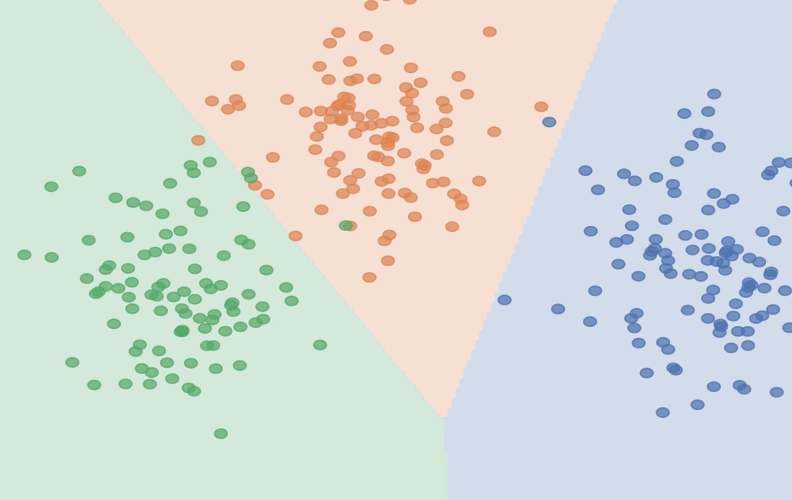
Linear Discriminant Evaluation (LDA) is a supervised studying approach used to floor the core elements, or patterns, within the information.
On this article we’re going to see how LDA works with a real-life instance, how it’s used to scale back the dimensionality of a dataset and determine class separation boundaries.
···
Linear Discriminant Evaluation is a statistical approach, usually utilized within the information preparation section of Machine Studying Classification issues [1]. It is used to scale back the dimensionality of a dataset, and spotlight the traits of the information that finest make sure the separability of its totally different lessons.
One main utility of LDA, for example, is in picture classification[2]. Picture classification datasets are inclined to have 1000’s of options and LDA is used to scale back the variety of options that can be utilized to correctly distinguish between lessons, after which run a classification machine studying algorithm on a a lot smaller function house.
Linear Discriminant Evaluation: the approach
In literature, LDA can be known as Regular Discriminant Evaluation or Fisher Linear Discriminant Evaluation, the latter being a reference to Ronald A. Fisher, the polymath who developed the criterion LDA goals to maximise.
Fisher’s Criterion: the ratio of between-class and within-class variance [2]
The purpose
The thought behind LDA is to take a dataset with high-dimensionality, e.g., a dataset with a whole lot or 1000’s of options, and characterize that very same dataset with a smaller variety of options.
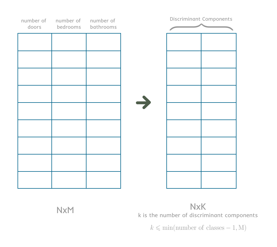
After making use of LDA, you do not essentially have options, you will have totally different linear discriminants, which nonetheless encode the unique traits of the information.
This latter level is essential. This system will cut back the quantity of data that’s used to describe the unique dataset, as a result of initially you had a considerable amount of options and afterwards you’ve gotten perhaps a handful of discriminant elements. Nonetheless, the traits of the unique dataset are preserved, that means, the dataset is simply encoded in a a lot smaller function house.
It is nearly like you’ve gotten a brilliant complicated music piece, with tons of notes for various devices after which convert it to MIDI, which is encoded and transmitted in 8-bit bytes. However, within the MIDI model you are still in a position to distinguish the melody. The bones, i.e., the core traits of that music piece are nonetheless there, they’re simply encoded in a lower-dimensionality house.
Moreover, LDA ensures the totally different lessons within the dataset are as distinguishable as potential, such that you simply’re in a position to separate the information factors in every class as a lot as potential.
Assumptions
Earlier than leaping into the mathematical definition, it is vital to say that LDA should take into consideration a number of assumptions:
-
Information is linearly separable
-
Information follows a Gaussian (Regular) Distribution
-
Shared Covariance matrix throughout all lessons
Information is linearly separable
It is a very sturdy assumption for this method, the identify provides it away, Linear Discriminant Evaluation.
If you happen to try to use LDA to a dataset that isn’t linearly separable, i.e., the boundaries between the lessons within the information are curves and never traces, you could get discriminants, however they will not be the most effective encoding of the core traits of the dataset. LDA is thought to fail to correctly seize nonlinear relationships and manifold constructions within the information[3].
Information follows a Gaussian (Regular) Distribution
This system assumes that information from every class is drawn from a Gaussian Distribution, i.e., the Regular Distribution[4].
Shared Covariance matrix throughout all lessons
So as to maximize the separability between lessons, LDA wants to take a look at the variance within the information. Nonetheless, since we’re working with high-dimensionality information, i.e., matrices, as an alternative of scalars, we will not use the variance because the measure of unfold or dispersion. We have to use a covariance matrix.
Succinctly, the covariance matrix describes the quantity of unfold every function has, alongside its diagonal, in addition to, the correlation between every pair of options, on the off diagonal.
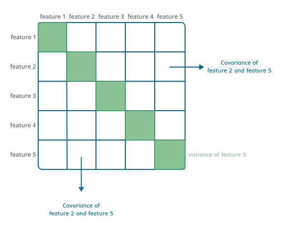
Particularly for LDA, the idea is there is a shared variance throughout all lessons, that means that every within-class covariance matrix is identical throughout all lessons. That is obligatory to make sure the pooled, i.e., shared, within-class covariance matrix is an correct illustration of every inside class covariances[5].
Mathematical Definition
Mathematically talking, Linear Discriminant Evaluation identifies the linear mixture of options that finest discriminate or distinguish between lessons within the information[5].
This methodology approximates the Bayes Classifier [6], which assigns an commentary to a category for which the posterior chance, i.e., the chance the commentary belongs to a category ok, is the best.
Recapping the Bayes Theorem:
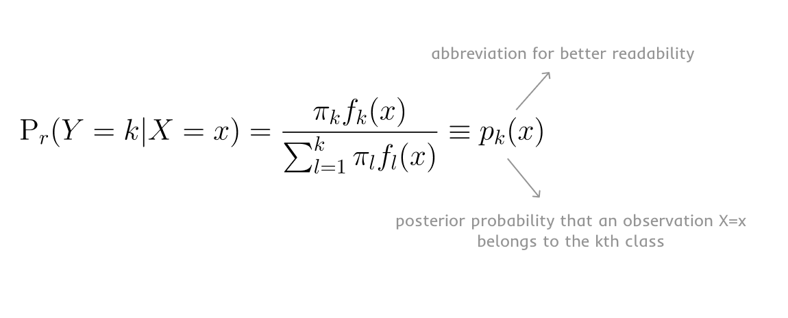
Let’s unpack this. Within the formulation above we’ve got:
-
Y – the label, i.e., the qualitative response variable
-
Ok – complete variety of lessons, i.e., labels, within the information
-
ok – particular person occasion of a category within the information
-
Pi_k- prior chance {that a} randomly chosen commentary comes from class ok
-
fk(x) – density operate of X for an commentary that comes from class ok. It is the chance of X given Y = ok , solely as a result of we’re working with a qualitative random variable X
Since we’re assuming the information follows a Gaussian Distribution, we are able to replace the overall Bayes Theorem formulation above and substitute the density operate placeholder, for the density operate of the Gaussian Distribution.
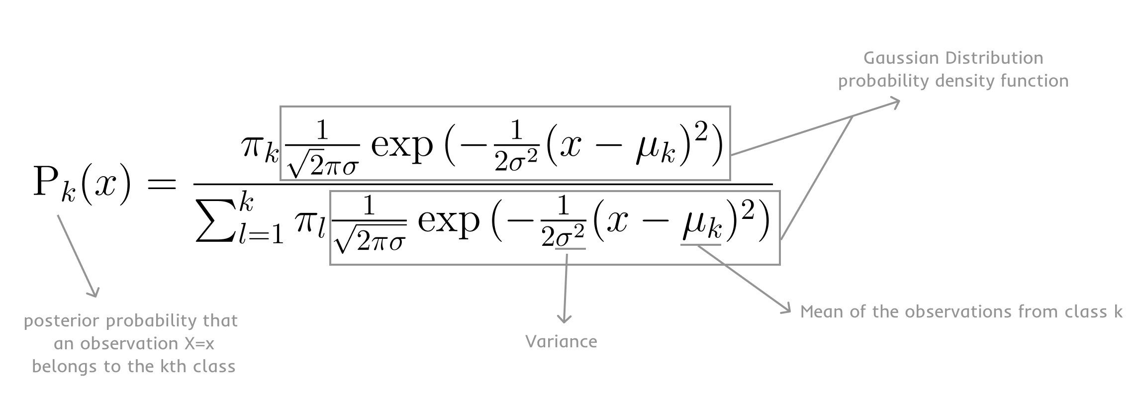
Trying on the formulation above, you’ll be able to inform it’s a bit verbose. So, taking the logarithm of the whole formulation and doing a little algebra, you get a way more concise definition of the posterior chance that an commentary X=x belongs to the kth class.
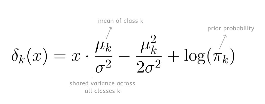
The Bayes Classifier will assign an commentary to a category the place the amount above, posterior chance, is the most important.
This sounds similar to what Linear Discriminant Evaluation does!
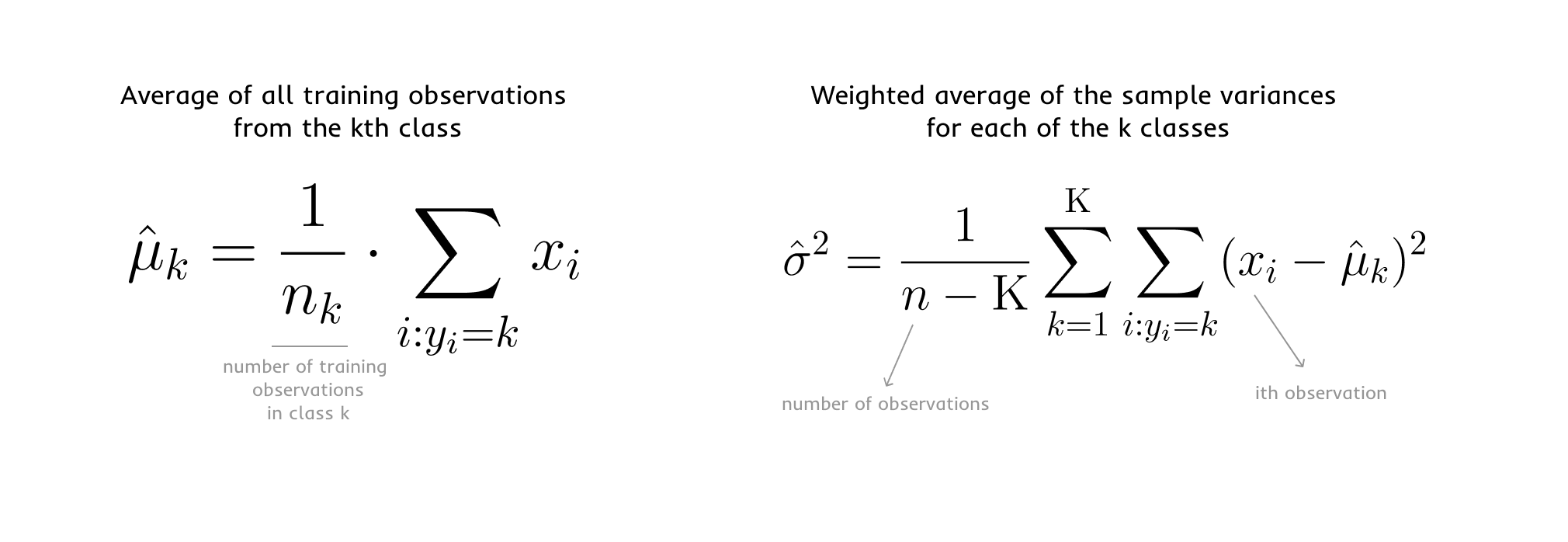
And that is the proper instinct, as a result of LDA takes the Bayes Classifier and approximates it by explicitly utilizing estimates for:
-
Prior chance
-
Imply of sophistication ok
-
Shared covariance throughout all ok lessons
Lastly, if we do not have details about the true prior chance, we are able to estimate it primarily based on the proportion of the coaching observations that belong to class ok.
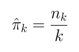
If you happen to’re ever doubtful in case you’re coping with the true amount or an estimator, word that, in algebra and statistics, the estimators at all times have a hat (^).
Placing all of it collectively, after taking into consideration all the required assumptions and the Bayes approximation, the LDA algorithm calculates the discriminant operate for every particular person information level x of the Gaussian variable X (X=x) and for every class ok. It can solely assign x to the category for which the discriminant operate is the most important:
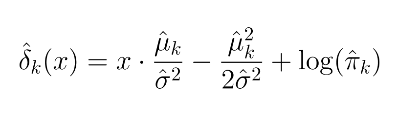
So, in the long run, the discriminant operate should be a linear operate of x.
However this formulation above was for the precise case after we solely have one predictor, the place x is a scalar, i.e., only a quantity.
In the kind of issues LDA is utilized to, there are usually a whole lot or 1000’s of predictors, i.e., options. We’re not working with scalars, however with matrices. Typically very massive, sparse matrices.
The Multivariate Gaussian variable X takes the next form:

The place every information level x is a row vector 1xN, following the Gaussian Distribution, the place N is the variety of predictors and is bigger than 1. Once you put all the information coaching information factors collectively, you’ve gotten the coaching dataset, a matrix.
Since we’re working with a Multivariate Gaussian Distribution the chance density operate is
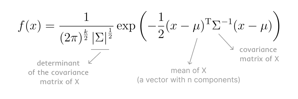
Once more, this can be a bit verbose. Following the identical algebra as earlier than, we are able to simplify this operate a bit and procure the linear discriminant operate for the multivariate case.
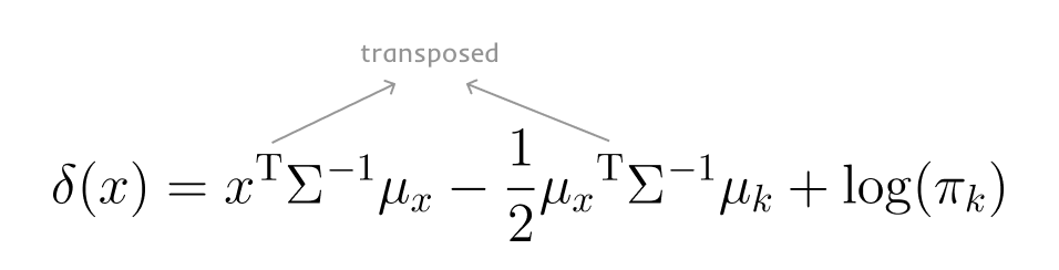
Equally, the discriminant operate nonetheless must be a linear operate of X.
The LDA algorithm calculates the discriminant operate for every particular person row vector x and for every class ok. It can solely assign x to the category for which the discriminant operate is the most important.
Now, let’s take a step again from all this intricate math.
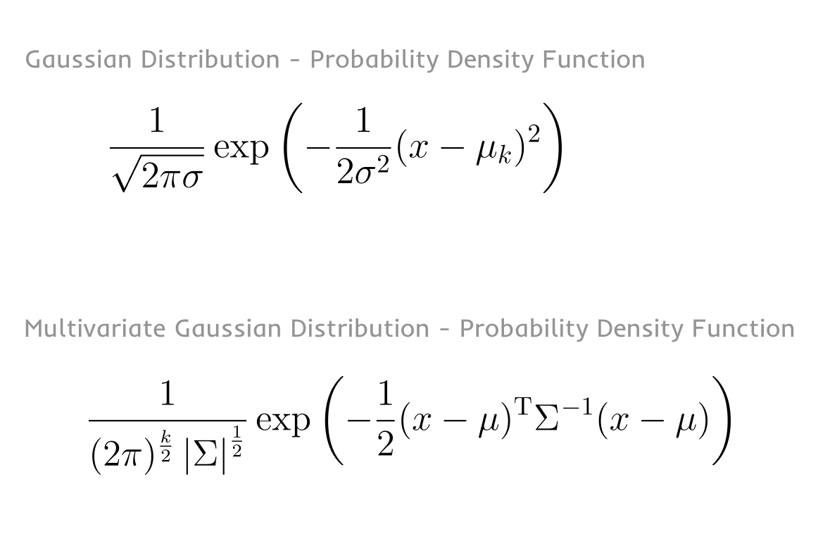
If you happen to examine the Bayes Classifier approximation formulation for the only predictor with the one for the multivariate predictor, the one predominant distinction is within the chance density operate of the distribution.
The why
Although this method is predicated on a statistical methodology developed within the Nineteen Thirties, there are a number of the reason why its utility remains to be very related at the moment:
-
Reduces computational complexity and energy (additionally saving cash)
-
Removes redundant options
-
Reduces overfitting
-
Facilitates visualization interpretability
Reduces computational complexity and energy
Operating a Machine Studying algorithm on a dataset with 1000’s of options may be computationally complicated, thus requiring specialised {hardware} like GPUs or TPUs, could take a very long time to run and, as a consequence, could value plenty of cash.
As fine-tuned or streamlined algorithms is likely to be, working commonplace matrix operations, similar to multiplication, inversion or eigenvectors and eigenvalues, on a 10×10 matrix tends to be computationally cheaper than working the identical operations on a 100×100, 1000×1000 or 10000×10000 matrix.
So, decreasing the dimensions of the matrix for computation, granted that the traits of the information are preserved, is a big benefit.
Removes redundant options
Since this method goals to reduce the within-class variance, whereas maximizing the between-class variance [3], it’s going to essentially give a decrease weight to all options that do not contribute to separate the lessons and can drop any options that redundant.
In the long run, the algorithm will take away these options that encode the identical data as different options which are extra related to tell apart between totally different lessons.
Reduces overfitting
When we’ve got a dataset with a lot of options, it is potential the classifier picks up the fallacious alerts, like noise within the information or correlations that do not essentially assist distinguish between the totally different lessons. However as a result of these alerts are so sturdy, the classifier can overfit to these alerts.
Since LDA reduces the dimensionality of the dataset, retaining the elements that finest encode the traits of the information and, as talked about above, additionally removes redundant options, it will possibly assist cut back overfitting.
Facilitates visualization interpretability
Linear dimensionality discount strategies similar to LDA are inclined to protect information interpretability, as a result of they challenge the information into discriminant features which are a linear mixture of the unique options. That means, the linear discriminants characterize the axes that finest separate the information factors into the totally different lessons. This enables for a direct mapping of the function contributions and for a greater understanding of the outcomes [3].
For the reason that information is projected in a lower-dimensionality house, it is also potential to raised visualize the separation between lessons.
Earlier than making use of LDA, it may need been onerous to plot the information because of the massive variety of options. Publish-LDA, with the information encoded into elements that may map to teams of options as an alternative of being 1:1 with every function, it is doubtless you’ll be able to plot the information in such a approach that’s potential to simply visualize the separation between lessons.
Limitations
Like some other approach, this one additionally has its limitations.
LDA’s predominant limitations are related to its assumptions.
With the sturdy linearity assumption, it isn’t the most effective approach for noisy or sparse information and will not present probably the most correct outcomes on classification issues with non-linear choice boundaries or distributions that aren’t Gaussian[4].
The estimation of the covariance matrix, particularly in high-dimensional information may pose limitations. When the variety of options is comparatively massive, in comparison with the variety of observations, the covariance matrix can have a excessive estimation variance and trigger efficiency points, even when all different assumptions maintain [4].
Linear Discriminant Evaluation (LDA) vs Principal Part Evaluation (PCA)
When interested by statistical strategies to scale back the dimensionality of a dataset, one other very talked-about approach could come to thoughts, the Principal Part Evaluation.
Though yow will discover similarities between them, there’s one putting distinction. LDA is a supervised methodology, that means, it makes use of the details about the options and the lessons/labels related to every information level when it is calculating the discriminants, whereas PCA does not [7]. Given this distinction Linear Discriminant Evaluation tends to be a way more strong methodology for dimensionality discount [2].
Each strategies are used to scale back the dimensionality of a dataset and, in the long run, each produce the axes or the course vectors which are used to challenge the unique dataset into the diminished dimension house.
The excellence between the 2 strategies is available in the truth that PCA computes the eigenvectors and ranks them by the related eigenvalues which have the most important variance, whereas LDA computes the eigenvectors that finest discriminate between lessons.
One other distinction between PCA and LDA refers back to the variety of non-zero eigenvectors that may be calculated. Within the case of PCA these are tied to the Principal Elements and, in LDA, to the Linear Discriminants.
There’s a most of Ok-1 Linear Discriminants that may be calculated in LDA, with Ok being the variety of lessons[8]. In observe the LDA algorithm calculates all of the totally different eigenvectors, however solely Ok-1 are non-zero.
Then again, PCA does not have this limitation.
Briefly, we’ve got that PCA, being an unsupervised methodology, produces the Principal Elements, i.e., the course vectors, that finest describe the unique dataset. Then again LDA, being a supervised methodology, produces the Linear Discriminants that finest discriminate, or separate the information, among the many totally different lessons [7].
LDA real-life instance
If you happen to’ve learn my article on Principal Part Evaluation, you will be aware of this instance.
Your buddy Maggie is a real-estate agent and needs some onerous information about what actually distinguishes the properties she has offered. So she asks you, her Information Scientist buddy, to assist with this job.
As at all times, step one is to check out the dataset at hand, utilizing the next Python code.
The output is a pleasant peek on the information.
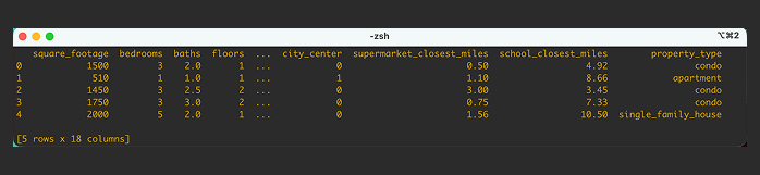
At this level you are simply getting aware of the totally different options, similar to:
-
square_footage – sq. footage for the property
-
bedrooms – variety of bedrooms within the property
-
baths – variety of baths within the property
-
…
And with the dataset label, property_type. There are three potential values for the dataset label: condo, condominium, single_family_house.
With so many options, it is actually onerous to pinpoint and even visualize how the information is unfold throughout the several types of properties.
That is whenever you keep in mind you need to use Linear Discriminant Evaluation to each visualize how the information in regards to the totally different property seems like, that means, are the information factors about condos all clustered collectively and much aside from the information factors for single household homes or residences?
On the identical time, you’ll have the ability to get extra details about what distinguishes the several types of properties within the dataset.
You instantly consider using the LinearDiscriminantAnalysis operate from ScikitLearn, and also you begin placing your code collectively.
You’ve your information imported from CSV right into a Pandas DataFrame for manipulation. Then separate between the options (X) and the labels (y), which goes for use later within the becoming of the classifier.
One factor you additionally take into account is to visualise the Covariance Matrix of the dataset, so you’ll be able to see the covariance between pairs of options. Since you recognize upfront you wish to do that and, acknowledging plenty of options are in numerous scales, you first normalize the function matrix X.
Discover that on the prime, there was no want to separate the information into coaching and testing. Maggie’s questions usually are not tied to predicting the kind of property a brand new, by no means seen earlier than, information level corresponds to. So you do not really want to separate the information, you utilize all of it to suit the LinearDiscriminantAnalysis operate.
With the LinearDiscriminantAnalysis utilized to the dataset, one of many stuff you examine is the coaching accuracy of ~98%.

In the long run, the information normalization will not make any distinction whenever you match the LinearDiscriminantAnalysis. It can simply make it simpler to visualise the Covariance Matrix with the next code.
The output is that this colourful matrix with the variance or unfold of every function on the diagonal and the correlation between options on the on the off diagonal.
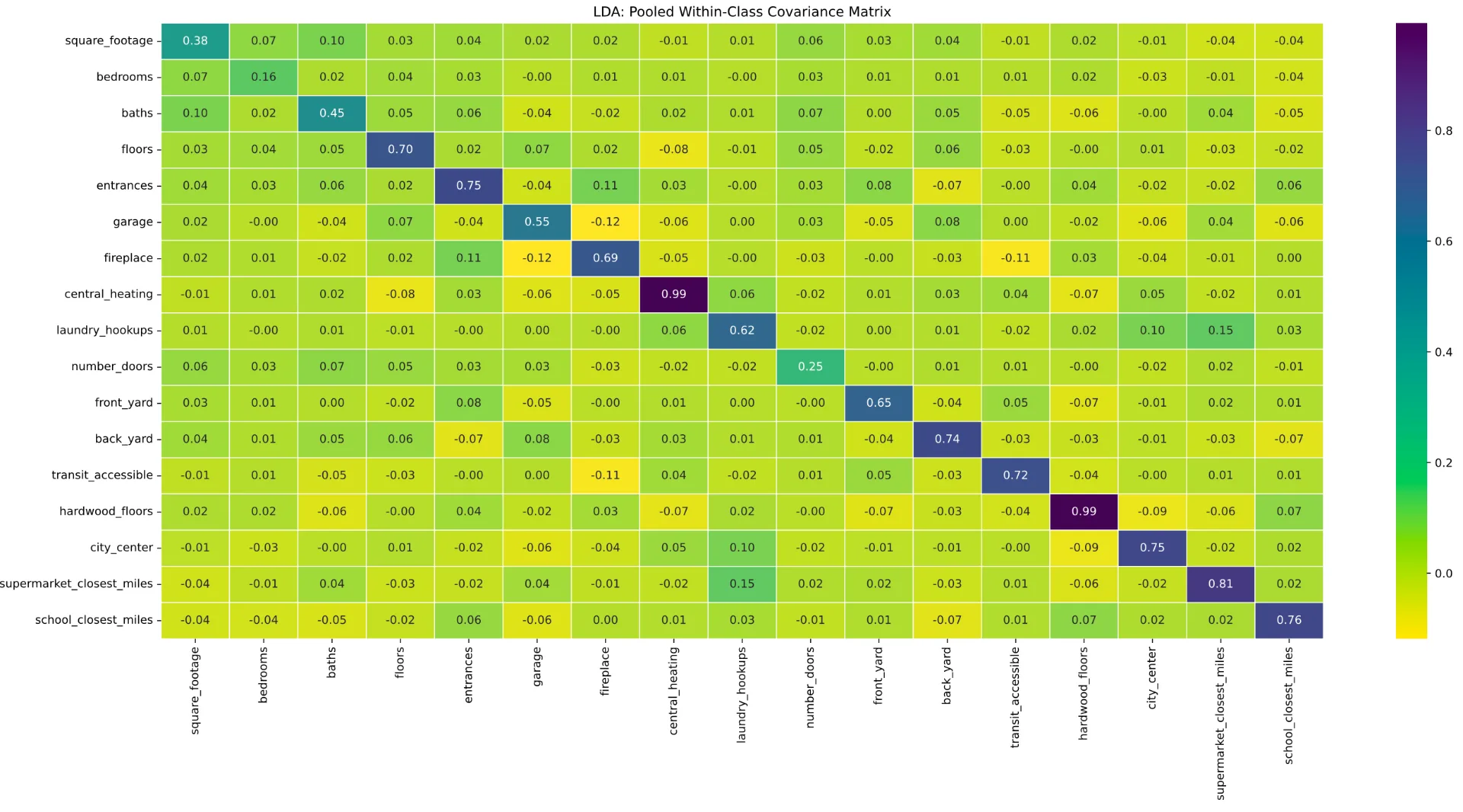
That is nice! Would not essentially reply Maggie’s query, however it’s good to examine, from an information exploration perspective. Particularly to identify examine options which are extremely correlated with one another.
Again to Maggie’s questions.
First she was concerned about understanding if information factors about condos all clustered collectively and much aside from the information factors for single household homes or residences.
That is one thing we are able to attempt to visualize after decreasing the dimensionality of the dataset.
You already match the LinearDiscriminant, so now you should plot the information factors within the two Linear Discriminants and colour them primarily based on their corresponding label.
So, you add a brand new operate to your codebase.
The output is that this plot, the place you’ll be able to see there is a extra marked separation between residences and single household homes and classification-wise, on this dataset a condominium is nearer to a single household home than to an condo.
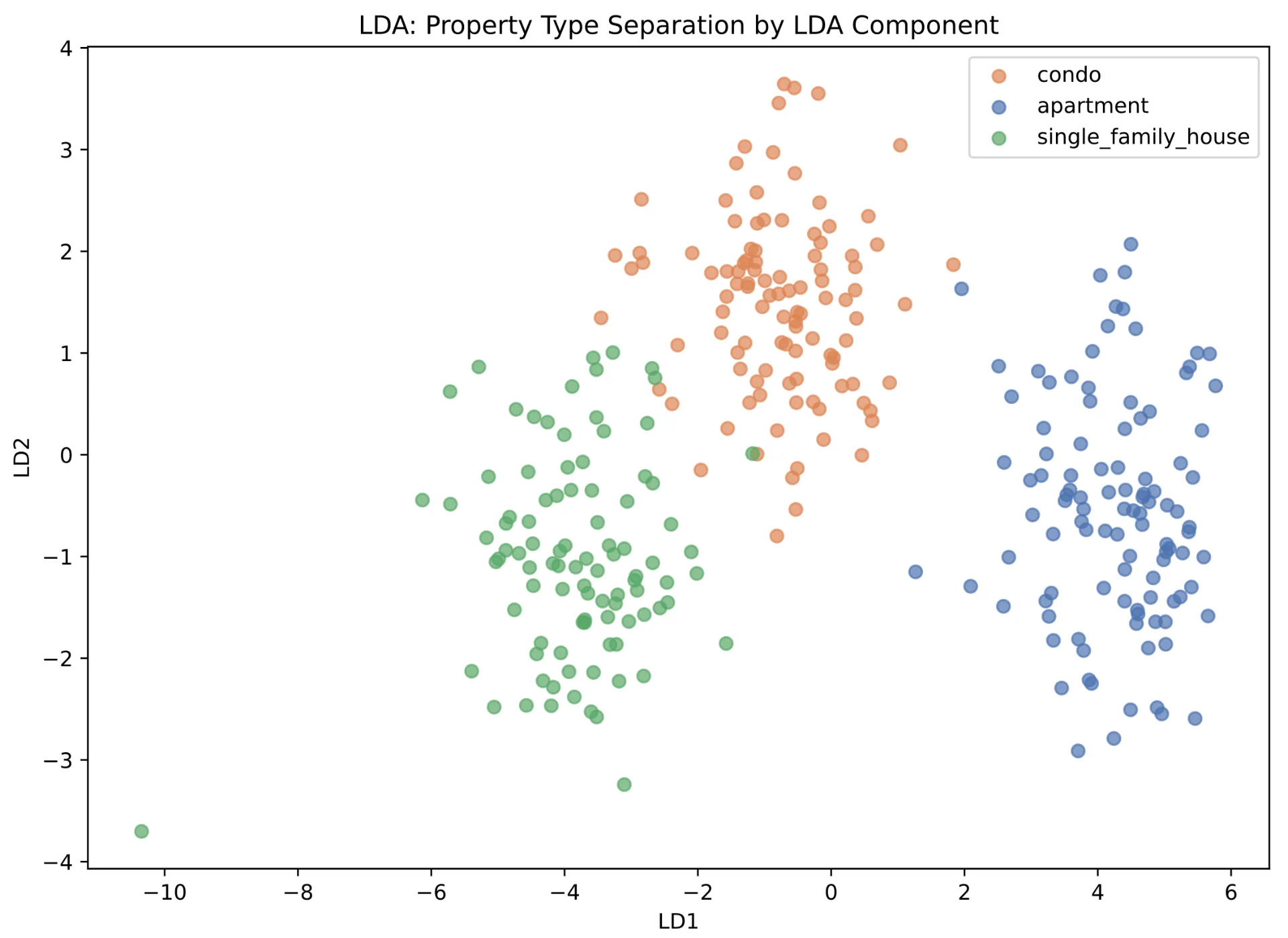
This plot is actually nice as a result of, you began off with a dataset with 17 options and three lessons. As you’ll be able to think about it will be very troublesome to visualise the structure of the information and the separation between lessons primarily based on 17 options. You may plot every pair of options towards one another, however it will by no means be a full image.
With LDA, you diminished the dimensionality to 2 Linear Discriminants which, on this case, is the utmost variety of elements you possibly can have. The utmost variety of Linear Discriminants is the minimal between the variety of options and the variety of lessons minus one. On this case, variety of lessons minus one wins, and also you picked n_components = 2.
That is very helpful, as a result of a 2D plot is one thing most individuals are used to interpret, and can assist Maggie actually get a greater image of the separation between the several types of properties.
However you are an information scientist and typically like to point out how one can make your visualizations shine. On this case, you wish to do that by including the choice boundary that separates every class. It can elevate your visualization and present Maggie you are actually as much as the duty!
So that you create a brand new operate, related because the one for the LinearDiscriminant plot, however the place you draw a mesh the place you will draw the factors that make up every choice boundary.
This actually pushes the earlier visualization to a different degree!
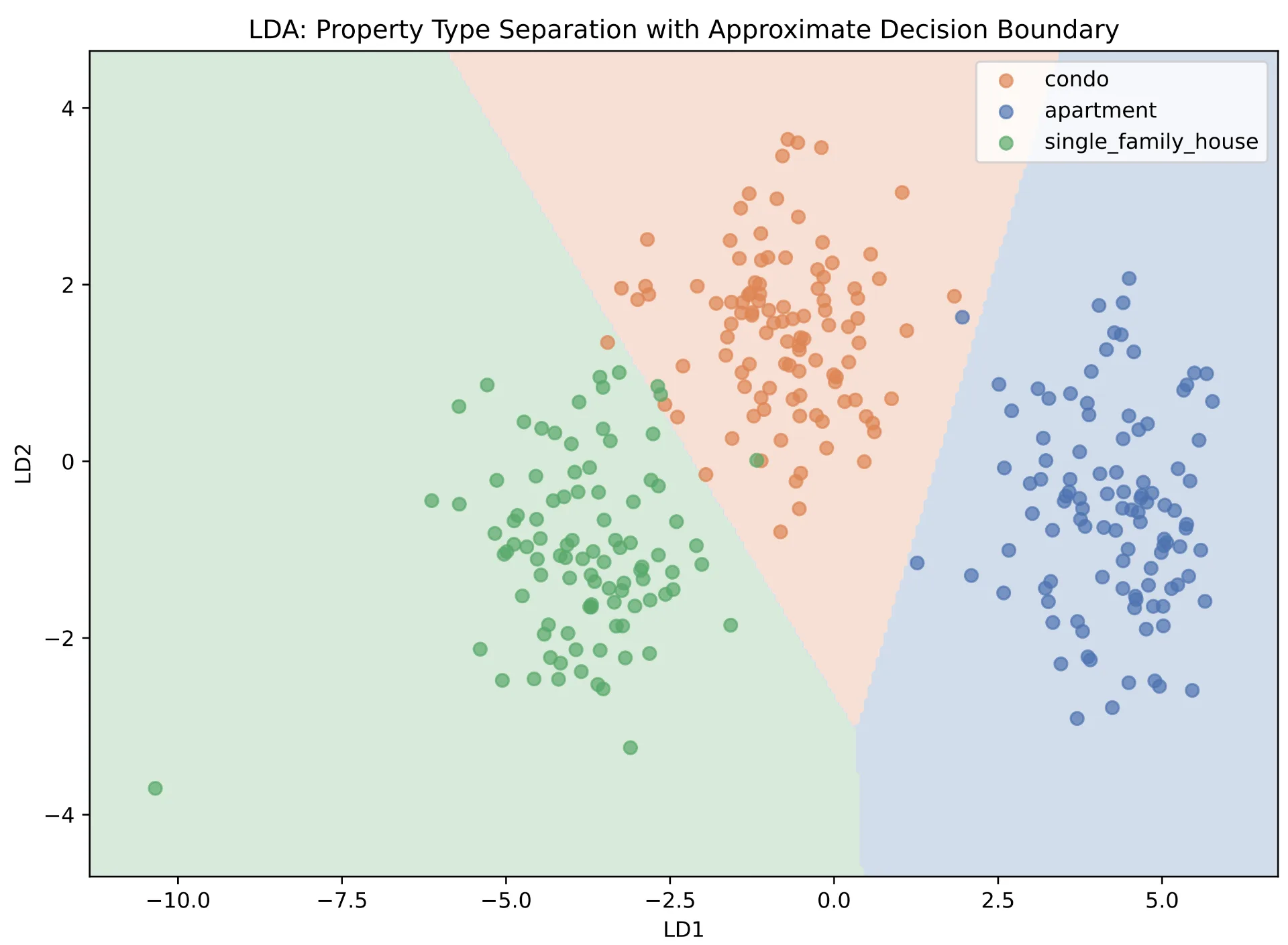
The choice boundaries you have drawn are technically approximate choice boundaries. The true choice boundaries come from the unique dataset, whereas these have been drawn primarily based on the information within the LinearDiscriminant. In observe, they’re very near the true choice boundaries for the reason that Linear Discriminants nonetheless encode the primary traits of the information. Nonetheless, it is vital to make this distinction.
Now, onto Maggie’s final query: What distinguishes the several types of properties within the dataset?
So as to reply this query you should flip to the dataset options and see what they’ll let you know about what distinguishes every class.
So that you begin searching for methods to get to details about the function contribution. You gladly keep in mind making use of the parameter solver=’eigen’ within the LinearDiscriminantAnalysis operate, it means the operate utilizing eigenvector decomposition to search out the linear discriminants that point out class separation.
Meaning you’ve gotten entry to the attribute scalings of the LinearDiscriminantAnalysis operate from ScikitLearn and examine how a lot every function contributes to every LinearDiscriminant
By default, scalings will output all of the potential eigenvectors, throughout all options. On this case, you will have one eigenvector for every of 17 options within the dataset.
Nonetheless, you set n_component = 2 within the LinearDiscriminantAnalysis operate, these are the one Linear Discriminants which are going for use to challenge the information right into a lower-dimensionality, i.e., from the 17 options to 2 Linear Discriminants which encode the core data of these options.
So as to output solely the 2 Linear Discriminants, as an alternative of all potential eigenvectors, you simply must truncate the scalings within the plot_class_separation_features.
This fashion the output is restricted to simply the 2 linear discriminants.
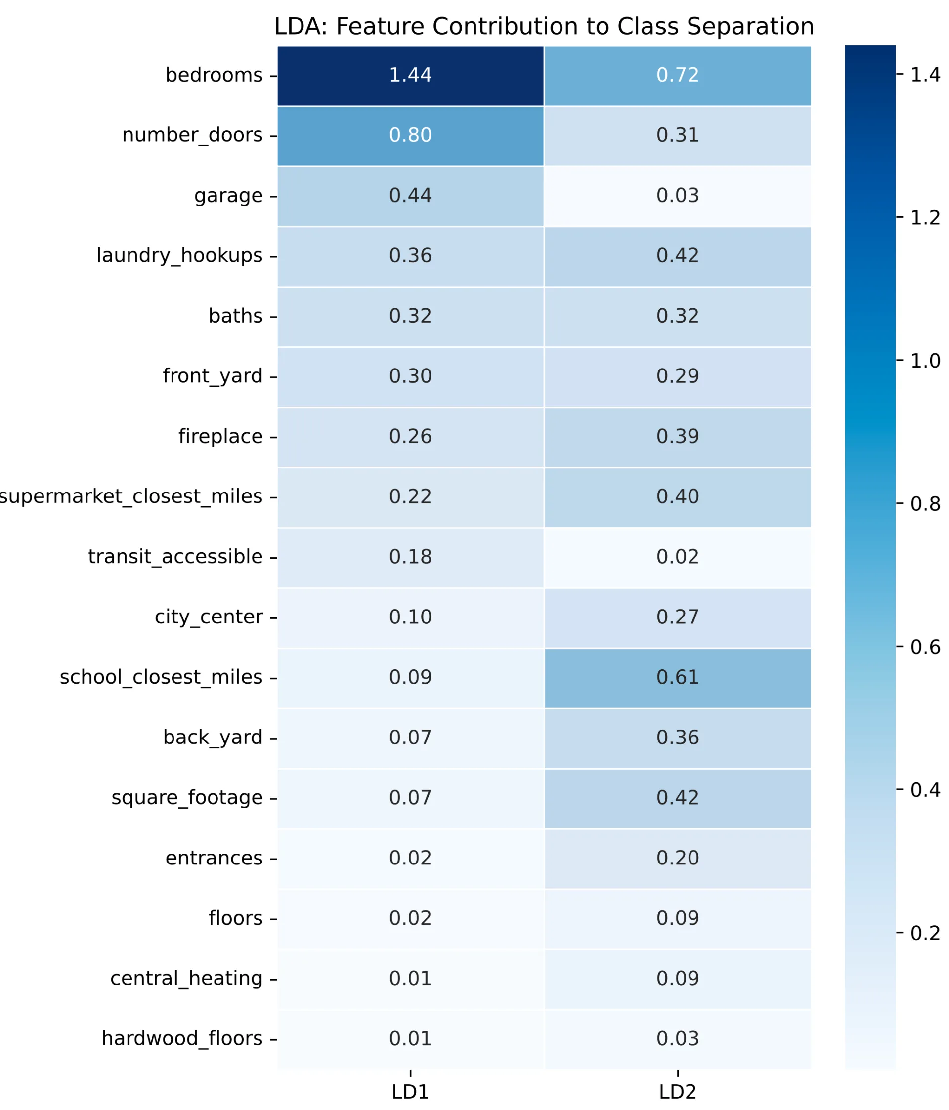
One thing that jumps immediately is the dimensions. Certainly you’ll be able to see that bedrooms is the function that, individually, contributes probably the most to every linear discriminant. Nonetheless, it is a bit onerous to interpret as a result of this isn’t a 0-100% scale. As an alternative these values are relative to one another and are primarily based on the uncooked values of the eigenvector decomposition.
To higher perceive how every function contributes to every Linear Discriminant, you determine to normalize the values in every linear discriminant column. The full contribution of all options in the direction of every particular person linear discriminant will complete to 100%.
To maintain issues separate, you create a brand new operate, in all much like the one you simply created, however it normalizes the values of the output of scalings.
In the long run, the rankings of how a lot every function contributes to every linear discriminant is identical however, making it such that the sum of all contributions inside every linear discriminant sum to 100% is a reassuring and undoubtedly a lot simpler to interpret.
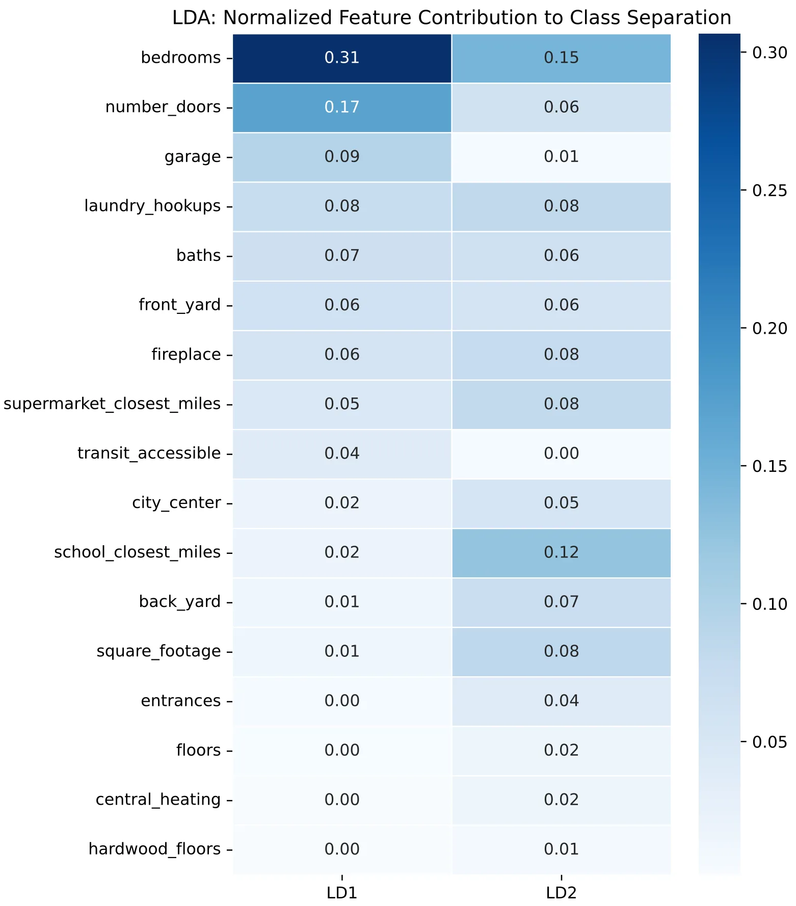
Initially, for the second linear discriminant, the primary and second highest function contributions have been for:
-
bedrooms = 0.72
-
school_closest_miles = 0.61
Which looks as if there was a barely vital distinction between them.
Publish-normalization you’ll be able to see that, in the direction of the second linear discriminant, the contribution of bedrooms is 0.15 in comparison with 0.12 for school_closest_miles. Would not seem to be such a large hole as earlier than.
Sadly this method does not will let you examine function significance throughout Linear Discriminants, however there’s nonetheless a method to piece collectively totally different data the Linear Discriminant Evaluation gives and reply Maggie’s query: What distinguishes the several types of properties within the dataset?
One you’ll be able to examine to reply this query is the Defined Variance, because it gives the ratio of how a lot of the separation between lessons is defined by every element. You simply must output the explained_variance_ratio_ attribute from the LinearDiscriminantAnalysis classifier.
You have been already anticipating that the primary Linear Discriminant can be the one which explains the best quantity of variation, for the reason that first one is at all times the one with the higherst eigenvalue. And you’ll see the large delta between the defined variability from the primary to the second Linear Discriminants.

The primary Linear Discriminant explains roughly 90% of the separation between lessons!
With this data together with the information from function contribution in the direction of the primary Linear Discriminant, it isn’t 100% bullet proof, however you’ll be able to intuit which options will are inclined to weigh extra in the direction of the separation between lessons.
You possibly can intuit that bedrooms, storage and laundry_hookups are the options that contribute probably the most to the separation between lessons, since they’re the options with the best significance in the direction of the primary Linear Discriminant and we all know that the primary Linear Discriminant contributes roughly 90% to the excellence between lessons.
With the choice boundary plot and this details about function contribution, you may get again to Maggie and share the insights in regards to the properties she offered!
···
Hope you loved studying about Linear Discriminant Evaluation. It is a very fascinating and highly effective statistical approach, used as an information preparation step for Classification issues in Machine Studying.
Thanks for studying!
References
-
C. Gambella, B. Ghaddar, and J. Naoum-Sawaya, “Optimization issues for machine studying: A survey,” European Journal of Operational Analysis, vol. 290, no. 3, pp. 807–828, Might 2021.
-
Wani AA. “Complete evaluate of dimensionality discount algorithms: challenges, limitations, and modern options,” PeerJ Comput. Sci., vol. 11, p. e3025, 2025, doi: 10.7717/peerj-cs.3025.
-
S. Gardner-Lubbe, “Linear discriminant evaluation for a number of purposeful information evaluation,” J. Appl. Stat., vol. 48, no. 11, pp. 1917–1933, 2021, doi: 10.1080/02664763.2020.1780569.
-
T. Hastie, R. Tibshirani, and J. Friedman, The Components of Statistical Studying: Information Mining, Inference, and Prediction, 2nd ed. New York, NY, USA: Springer, 2009
-
A. M. Martinez and A. C. Kak, “PCA versus LDA,” IEEE Transactions on Sample Evaluation and Machine Intelligence, vol. 23, no. 2, pp. 228-233, Feb. 2001, doi: 10.1109/34.908974
-
C. M. Bishop, Sample Recognition and Machine Studying. New York, NY, USA: Springer, 2006