Linear Regression in Time Sequence: Sources of Spurious Regression

1. Introduction

What is especially shocking is that the majority econometric textbooks warn in regards to the hazard of autocorrelated errors, but this concern persists in lots of printed papers. Granger and Newbold (1974) recognized a number of examples. As an illustration, they discovered printed equations with R² = 0.997 and the Durbin-Watson statistic (d) equal to 0.53. Probably the most excessive discovered is an equation with R² = 0.999 and d = 0.093.

It’s particularly problematic in economics and finance, the place many key variables exhibit autocorrelation or serial correlation between adjoining values, notably if the sampling interval is small, resembling every week or a month, resulting in deceptive conclusions if not dealt with accurately. For instance, as we speak’s GDP is strongly correlated with the GDP of the earlier quarter. Our put up offers an in depth clarification of the outcomes from Granger and Newbold (1974) and Python simulation (see part 7) replicating the important thing outcomes offered of their article.

Whether or not you’re an economist, knowledge scientist, or analyst working with time sequence knowledge, understanding this concern is essential to making sure your fashions produce significant outcomes.

To stroll you thru this paper, the subsequent part will introduce the random stroll and the ARIMA(0,1,1) course of. In part 3, we are going to clarify how Granger and Newbold (1974) describe the emergence of nonsense regressions, with examples illustrated in part 4. Lastly, we’ll present how you can keep away from spurious regressions when working with time sequence knowledge.

2. Easy presentation of a Random Stroll and ARIMA(0,1,1) Course of

2.1 Random Stroll

Let 𝐗ₜ be a time sequence. We are saying that 𝐗ₜ follows a random stroll if its illustration is given by:

𝐗ₜ = 𝐗ₜ₋₁ + 𝜖ₜ. (1)

The place 𝜖ₜ is a white noise. It may be written as a sum of white noise, a helpful kind for simulation. It’s a non-stationary time sequence as a result of its variance is dependent upon the time t.

2.2 ARIMA(0,1,1) Course of

The ARIMA(0,1,1) course of is given by:

𝐗ₜ = 𝐗ₜ₋₁ + 𝜖ₜ − 𝜃 𝜖ₜ₋₁. (2)

the place 𝜖ₜ is a white noise. The ARIMA(0,1,1) course of is non-stationary. It may be written as a sum of an impartial random stroll and white noise:

𝐗ₜ = 𝐗₀ + random stroll + white noise. (3) This way is helpful for simulation.

These non-stationary sequence are sometimes employed as benchmarks towards which the forecasting efficiency of different fashions is judged.

3. Random stroll can result in Nonsense Regression

First, let’s recall the Linear Regression mannequin. The linear regression mannequin is given by:

𝐘 = 𝐗𝛽 + 𝜖. (4)

The place 𝐘 is a T × 1 vector of the dependent variable, 𝛽 is a Ok × 1 vector of the coefficients, 𝐗 is a T × Ok matrix of the impartial variables containing a column of ones and (Ok−1) columns with T observations on every of the (Ok−1) impartial variables, that are stochastic however distributed independently of the T × 1 vector of the errors 𝜖. It’s usually assumed that:

𝐄(𝜖) = 0, (5)

and

𝐄(𝜖𝜖′) = 𝜎²𝐈. (6)

the place 𝐈 is the identification matrix.

A check of the contribution of impartial variables to the reason of the dependent variable is the F-test. The null speculation of the check is given by:

𝐇₀: 𝛽₁ = 𝛽₂ = ⋯ = 𝛽ₖ₋₁ = 0, (7)

And the statistic of the check is given by:

𝐅 = (𝐑² / (𝐊−1)) / ((1−𝐑²) / (𝐓−𝐊)). (8)

the place 𝐑² is the coefficient of dedication.

If we wish to assemble the statistic of the check, let’s assume that the null speculation is true, and one tries to suit a regression of the shape (Equation 4) to the degrees of an financial time sequence. Suppose subsequent that these sequence will not be stationary or are extremely autocorrelated. In such a state of affairs, the check process is invalid since 𝐅 in (Equation 8) will not be distributed as an F-distribution underneath the null speculation (Equation 7). In reality, underneath the null speculation, the errors or residuals from (Equation 4) are given by:

𝜖ₜ = 𝐘ₜ − 𝐗𝛽₀ ; t = 1, 2, …, T. (9)

And may have the identical autocorrelation construction as the unique sequence 𝐘.

Some concept of the distribution downside can come up within the state of affairs when:

𝐘ₜ = 𝛽₀ + 𝐗ₜ𝛽₁ + 𝜖ₜ. (10)

The place 𝐘ₜ and 𝐗ₜ observe impartial first-order autoregressive processes:

𝐘ₜ = 𝜌 𝐘ₜ₋₁ + 𝜂ₜ, and 𝐗ₜ = 𝜌* 𝐗ₜ₋₁ + 𝜈ₜ. (11)

The place 𝜂ₜ and 𝜈ₜ are white noise.

We all know that on this case, 𝐑² is the sq. of the correlation between 𝐘ₜ and 𝐗ₜ. They use Kendall’s outcome from the article Knowles (1954), which expresses the variance of 𝐑:

𝐕𝐚𝐫(𝐑) = (1/T)* (1 + 𝜌𝜌*) / (1 − 𝜌𝜌*). (12)

Since 𝐑 is constrained to lie between -1 and 1, if its variance is larger than 1/3, the distribution of 𝐑 can’t have a mode at 0. This means that 𝜌𝜌* > (T−1) / (T+1).

Thus, for instance, if T = 20 and 𝜌 = 𝜌*, a distribution that’s not unimodal at 0 will probably be obtained if 𝜌 > 0.86, and if 𝜌 = 0.9, 𝐕𝐚𝐫(𝐑) = 0.47. So the 𝐄(𝐑²) will probably be near 0.47.

It has been proven that when 𝜌 is near 1, 𝐑² may be very excessive, suggesting a powerful relationship between 𝐘ₜ and 𝐗ₜ. Nonetheless, in actuality, the 2 sequence are utterly impartial. When 𝜌 is close to 1, each sequence behave like random walks or near-random walks. On high of that, each sequence are extremely autocorrelated, which causes the residuals from the regression to even be strongly autocorrelated. In consequence, the Durbin-Watson statistic 𝐝 will probably be very low.

For this reason a excessive 𝐑² on this context ought to by no means be taken as proof of a real relationship between the 2 sequence.

To discover the potential for acquiring a spurious regression when regressing two impartial random walks, a sequence of simulations proposed by Granger and Newbold (1974) will probably be performed within the subsequent part.

4. Simulation outcomes utilizing Python.

On this part, we are going to present utilizing simulations that utilizing the regression mannequin with impartial random walks bias the estimation of the coefficients and the speculation checks of the coefficients are invalid. The Python code that can produce the outcomes of the simulation will probably be offered in part 6.

A regression equation proposed by Granger and Newbold (1974) is given by:

𝐘ₜ = 𝛽₀ + 𝐗ₜ𝛽₁ + 𝜖ₜ

The place 𝐘ₜ and 𝐗ₜ had been generated as impartial random walks, every of size 50. The values 𝐒 = |𝛽̂₁| / √(𝐒𝐄̂(𝛽̂₁)), representing the statistic for testing the importance of 𝛽₁, for 100 simulations will probably be reported within the desk under.

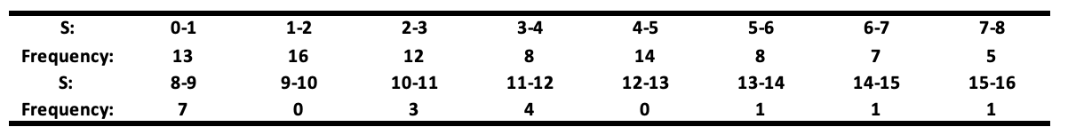
The null speculation of no relationship between 𝐘ₜ and 𝐗ₜ is rejected on the 5% degree if 𝐒 > 2. This desk reveals that the null speculation (𝛽 = 0) is wrongly rejected in a few quarter (71 instances) of all circumstances. That is awkward as a result of the 2 variables are impartial random walks, which means there’s no precise relationship. Let’s break down why this occurs.

If 𝛽̂₁ / 𝐒𝐄̂ follows a 𝐍(0,1), the anticipated worth of 𝐒, its absolute worth, ought to be √2 / π ≈ 0.8 (√2/π is the imply of absolutely the worth of a typical regular distribution). Nonetheless, the simulation outcomes present a median of 4.59, which means the estimated 𝐒 is underestimated by an element of:

4.59 / 0.8 = 5.7

In classical statistics, we normally use a t-test threshold of round 2 to test the importance of a coefficient. Nonetheless, these outcomes present that, on this case, you would want to make use of a threshold of 11.4 to correctly check for significance:

2 × (4.59 / 0.8) = 11.4

Interpretation: We’ve simply proven that together with variables that don’t belong within the mannequin — particularly random walks — can result in utterly invalid significance checks for the coefficients.

To make their simulations even clearer, Granger and Newbold (1974) ran a sequence of regressions utilizing variables that observe both a random stroll or an ARIMA(0,1,1) course of.

Right here is how they arrange their simulations:

They regressed a dependent sequence 𝐘ₜ on m sequence 𝐗ⱼ,ₜ (with j = 1, 2, …, m), various m from 1 to five. The dependent sequence 𝐘ₜ and the impartial sequence 𝐗ⱼ,ₜ observe the identical forms of processes, and so they examined 4 circumstances:

• Case 1 (Ranges): 𝐘ₜ and 𝐗ⱼ,ₜ observe random walks.
• Case 2 (Variations): They use the primary variations of the random walks, that are stationary.
• Case 3 (Ranges): 𝐘ₜ and 𝐗ⱼ,ₜ observe ARIMA(0,1,1).
• Case 4 (Variations): They use the primary variations of the earlier ARIMA(0,1,1) processes, that are stationary.

Every sequence has a size of fifty observations, and so they ran 100 simulations for every case.

All error phrases are distributed as 𝐍(0,1), and the ARIMA(0,1,1) sequence are derived because the sum of the random stroll and impartial white noise. The simulation outcomes, based mostly on 100 replications with sequence of size 50, are summarized within the subsequent desk.

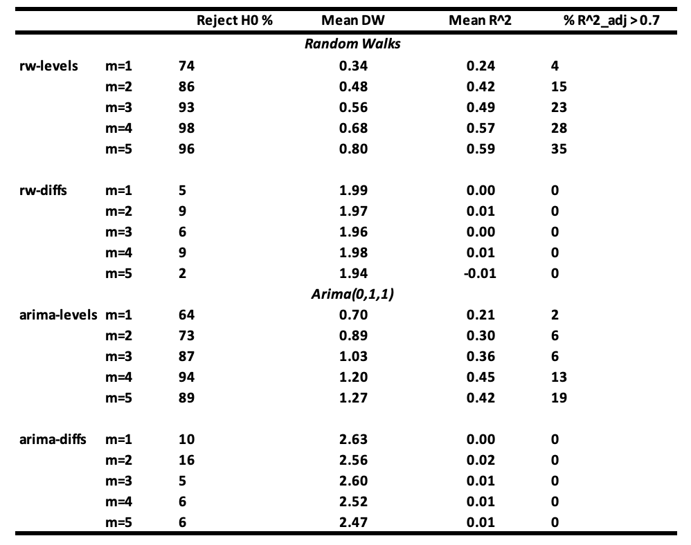
Interpretation of the outcomes :

• It’s seen that the chance of not rejecting the null speculation of no relationship between 𝐘ₜ and 𝐗ⱼ,ₜ turns into very small when m ≥ 3 when regressions are made with random stroll sequence (rw-levels). The 𝐑² and the imply Durbin-Watson improve. Related outcomes are obtained when the regressions are made with ARIMA(0,1,1) sequence (arima-levels).
• When white noise sequence (rw-diffs) are used, classical regression evaluation is legitimate because the error sequence will probably be white noise and least squares will probably be environment friendly.
• Nonetheless, when the regressions are made with the variations of ARIMA(0,1,1) sequence (arima-diffs) or first-order shifting common sequence MA(1) course of, the null speculation is rejected, on common:

(10 + 16 + 5 + 6 + 6) / 5 = 8.6

which is larger than 5% of the time.

In case your variables are random walks or near them, and also you embody pointless variables in your regression, you’ll usually get fallacious outcomes. Excessive 𝐑² and low Durbin-Watson values don’t verify a real relationship however as an alternative point out a probable spurious one.

5. Find out how to keep away from spurious regression in time sequence

It’s actually arduous to give you an entire checklist of the way to keep away from spurious regressions. Nonetheless, there are a number of good practices you may observe to decrease the chance as a lot as potential.

If one performs a regression evaluation with time sequence knowledge and finds that the residuals are strongly autocorrelated, there’s a significant issue with regards to decoding the coefficients of the equation. To test for autocorrelation within the residuals, one can use the Durbin-Watson check or the Portmanteau check.

Primarily based on the examine above, we are able to conclude that if a regression evaluation carried out with economical variables produces strongly autocorrelated residuals, which means a low Durbin-Watson statistic, then the outcomes of the evaluation are more likely to be spurious, regardless of the worth of the coefficient of dedication R² noticed.

In such circumstances, it is very important perceive the place the mis-specification comes from. Based on the literature, misspecification normally falls into three classes : (i) the omission of a related variable, (ii) the inclusion of an irrelevant variable, or (iii) autocorrelation of the errors. More often than not, mis-specification comes from a mixture of these three sources.

To keep away from spurious regression in a time sequence, a number of suggestions may be made:

• The primary suggestion is to pick the best macroeconomic variables which are more likely to clarify the dependent variable. This may be achieved by reviewing the literature or consulting consultants within the area.
• The second suggestion is to stationarize the sequence by taking first variations. Most often, the primary variations of macroeconomic variables are stationary and nonetheless simple to interpret. For macroeconomic knowledge, it’s strongly advisable to distinguish the sequence as soon as to cut back the autocorrelation of the residuals, particularly when the pattern dimension is small. There’s certainly typically sturdy serial correlation noticed in these variables. A easy calculation reveals that the primary variations will virtually all the time have a lot smaller serial correlations than the unique sequence.
• The third suggestion is to make use of the Field-Jenkins methodology to mannequin every macroeconomic variable individually after which seek for relationships between the sequence by relating the residuals from every particular person mannequin. The concept right here is that the Field-Jenkins course of extracts the defined a part of the sequence, leaving the residuals, which include solely what can’t be defined by the sequence’ personal previous habits. This makes it simpler to test whether or not these unexplained components (residuals) are associated throughout variables.

6. Conclusion

Many econometrics textbooks warn about specification errors in regression fashions, however the issue nonetheless reveals up in lots of printed papers. Granger and Newbold (1974) highlighted the chance of spurious regressions, the place you get a excessive paired with very low Durbin-Watson statistics.

Utilizing Python simulations, we confirmed a number of the fundamental causes of those spurious regressions, particularly together with variables that don’t belong within the mannequin and are extremely autocorrelated. We additionally demonstrated how these points can utterly distort speculation checks on the coefficients.

Hopefully, this put up will assist cut back the chance of spurious regressions in future econometric analyses.

7. Appendice: Python code for simulation.

#####################################################Simulation Code for desk 1 #####################################################

import numpy as np
import pandas as pd
import statsmodels.api as sm
import matplotlib.pyplot as plt

np.random.seed(123)
M = 100 
n = 50
S = np.zeros(M)
for i in vary(M):
#---------------------------------------------------------------
# Generate the information
#---------------------------------------------------------------
    espilon_y = np.random.regular(0, 1, n)
    espilon_x = np.random.regular(0, 1, n)

    Y = np.cumsum(espilon_y)
    X = np.cumsum(espilon_x)
#---------------------------------------------------------------
# Match the mannequin
#---------------------------------------------------------------
    X = sm.add_constant(X)
    mannequin = sm.OLS(Y, X).match()
#---------------------------------------------------------------
# Compute the statistic
#------------------------------------------------------
    S[i] = np.abs(mannequin.params[1])/mannequin.bse[1]


#------------------------------------------------------ 
#              Most worth of S
#------------------------------------------------------
S_max = int(np.ceil(max(S)))

#------------------------------------------------------ 
#                Create bins
#------------------------------------------------------
bins = np.arange(0, S_max + 2, 1)  

#------------------------------------------------------
#    Compute the histogram
#------------------------------------------------------
frequency, bin_edges = np.histogram(S, bins=bins)

#------------------------------------------------------
#    Create a dataframe
#------------------------------------------------------

df = pd.DataFrame({
    "S Interval": [f"{int(bin_edges[i])}-{int(bin_edges[i+1])}" for i in vary(len(bin_edges)-1)],
    "Frequency": frequency
})
print(df)
print(np.imply(S))

#####################################################Simulation Code for desk 2 #####################################################

import numpy as np
import pandas as pd
import statsmodels.api as sm
from statsmodels.stats.stattools import durbin_watson
from tabulate import tabulate

np.random.seed(1)  # Pour rendre les résultats reproductibles

#------------------------------------------------------
# Definition of capabilities
#------------------------------------------------------

def generate_random_walk(T):
    """
    Génère une série de longueur T suivant un random stroll :
        Y_t = Y_{t-1} + e_t,
    où e_t ~ N(0,1).
    """
    e = np.random.regular(0, 1, dimension=T)
    return np.cumsum(e)

def generate_arima_0_1_1(T):
    """
    Génère un ARIMA(0,1,1) selon la méthode de Granger & Newbold :
    la série est obtenue en additionnant une marche aléatoire et un bruit blanc indépendant.
    """
    rw = generate_random_walk(T)
    wn = np.random.regular(0, 1, dimension=T)
    return rw + wn

def distinction(sequence):
    """
    Calcule la différence première d'une série unidimensionnelle.
    Retourne une série de longueur T-1.
    """
    return np.diff(sequence)

#------------------------------------------------------
# Paramètres
#------------------------------------------------------

T = 50           # longueur de chaque série
n_sims = 100     # nombre de simulations Monte Carlo
alpha = 0.05     # seuil de significativité

#------------------------------------------------------
# Definition of perform for simulation
#------------------------------------------------------

def run_simulation_case(case_name, m_values=[1,2,3,4,5]):
    """
    case_name : un identifiant pour le sort de génération :
        - 'rw-levels' : random stroll (ranges)
        - 'rw-diffs'  : variations of RW (white noise)
        - 'arima-levels' : ARIMA(0,1,1) en niveaux
        - 'arima-diffs'  : différences d'un ARIMA(0,1,1) => MA(1)
    
    m_values : liste du nombre de régresseurs.
    
    Retourne un DataFrame avec pour chaque m :
        - % de rejets de H0
        - Durbin-Watson moyen
        - R^2_adj moyen
        - % de R^2 > 0.1
    """
    outcomes = []
    
    for m in m_values:
        count_reject = 0
        dw_list = []
        r2_adjusted_list = []
        
        for _ in vary(n_sims):
#--------------------------------------
# 1) Era of independents de Y_t and X_{j,t}.
#----------------------------------------
            if case_name == 'rw-levels':
                Y = generate_random_walk(T)
                Xs = [generate_random_walk(T) for __ in range(m)]
            
            elif case_name == 'rw-diffs':
                # Y et X sont les différences d'un RW, i.e. ~ white noise
                Y_rw = generate_random_walk(T)
                Y = distinction(Y_rw)
                Xs = []
                for __ in vary(m):
                    X_rw = generate_random_walk(T)
                    Xs.append(distinction(X_rw))
                # NB : maintenant Y et Xs ont longueur T-1
                # => ajuster T_effectif = T-1
                # => on prendra T_effectif factors pour la régression
            
            elif case_name == 'arima-levels':
                Y = generate_arima_0_1_1(T)
                Xs = [generate_arima_0_1_1(T) for __ in range(m)]
            
            elif case_name == 'arima-diffs':
                # Différences d'un ARIMA(0,1,1) => MA(1)
                Y_arima = generate_arima_0_1_1(T)
                Y = distinction(Y_arima)
                Xs = []
                for __ in vary(m):
                    X_arima = generate_arima_0_1_1(T)
                    Xs.append(distinction(X_arima))
            
            # 2) Prépare les données pour la régression
            #    Selon le cas, la longueur est T ou T-1
            if case_name in ['rw-levels','arima-levels']:
                Y_reg = Y
                X_reg = np.column_stack(Xs) if m>0 else np.array([])
            else:
                # dans les cas de différences, la longueur est T-1
                Y_reg = Y
                X_reg = np.column_stack(Xs) if m>0 else np.array([])
            
            # 3) Régression OLS
            X_with_const = sm.add_constant(X_reg)  # Ajout de l'ordonnée à l'origine
            mannequin = sm.OLS(Y_reg, X_with_const).match()
            
            # 4) Check international F : H0 : tous les beta_j = 0
            #    On regarde si p-value < alpha
            if mannequin.f_pvalue will not be None and mannequin.f_pvalue < alpha:
                count_reject += 1
            
            # 5) R^2, Durbin-Watson
            r2_adjusted_list.append(mannequin.rsquared_adj)
            
            
            dw_list.append(durbin_watson(mannequin.resid))
        
        # Statistiques sur n_sims répétitions
        reject_percent = 100 * count_reject / n_sims
        dw_mean = np.imply(dw_list)
        r2_mean = np.imply(r2_adjusted_list)
        r2_above_0_7_percent = 100 * np.imply(np.array(r2_adjusted_list) > 0.7)
        
        outcomes.append({
            'm': m,
            'Reject %': reject_percent,
            'Imply DW': dw_mean,
            'Imply R^2': r2_mean,
            '% R^2_adj>0.7': r2_above_0_7_percent
        })
    
    return pd.DataFrame(outcomes)
    
#------------------------------------------------------
# Software of the simulation
#------------------------------------------------------       

circumstances = ['rw-levels', 'rw-diffs', 'arima-levels', 'arima-diffs']
all_results = {}

for c in circumstances:
    df_res = run_simulation_case(c, m_values=[1,2,3,4,5])
    all_results[c] = df_res

#------------------------------------------------------
# Retailer knowledge in desk
#------------------------------------------------------

for case, df_res in all_results.objects():
    print(f"nn{case}")
    print(tabulate(df_res, headers='keys', tablefmt='fancy_grid'))

References

• Granger, Clive WJ, and Paul Newbold. 1974. “Spurious Regressions in Econometrics.” Journal of Econometrics 2 (2): 111–20.
• Knowles, EAG. 1954. “Workout routines in Theoretical Statistics.” Oxford College Press.