


mannequin fails not as a result of the algorithm is weak, however as a result of the variables weren’t ready in a manner the mannequin can correctly perceive?
In credit score danger modeling, we regularly give attention to mannequin selection, efficiency metrics, characteristic choice, or validation. However earlier than estimating any coefficient, one other query deserves consideration: how ought to every variable enter the mannequin?
A uncooked variable just isn’t all the time one of the best illustration of danger.
A steady variable might have a non-linear relationship with default. A categorical variable might comprise too many modalities. Some variables might embody outliers, lacking values, unstable distributions, or classes with only a few observations. If these points are ignored, the mannequin might grow to be unstable, troublesome to interpret, and fewer dependable in manufacturing.
That is the place categorization turns into essential.
Categorization, additionally known as coarse classification, grouping, classing, or binning, consists of remodeling uncooked variable values right into a smaller variety of significant teams. In credit score scoring, these teams usually are not created just for comfort. They’re created to make the connection between the variable and default danger clearer, extra steady, and simpler to make use of in a mannequin.
This step is especially helpful when the ultimate mannequin is a logistic regression, which stays extensively utilized in credit score scoring as a result of it’s clear, interpretable, and simple to translate right into a scorecard.
For categorical variables, categorization helps cut back the variety of modalities. For steady variables, it helps seize non-linear danger patterns, cut back the affect of outliers, deal with lacking values, enhance interpretability, and put together the variables for Weight of Proof transformation.
On this article, we’ll research why categorization is a necessary step in credit score scoring and the way it may be used to rework uncooked variables into steady danger courses.
In Part 1, we clarify why categorization is beneficial for each categorical and steady variables, particularly within the context of logistic regression.
In Part 2, we present tips on how to analyze the connection between steady variables and default danger utilizing graphical monotonicity evaluation.
In Part 3, we introduce the principle categorization strategies, together with equal-interval binning, equal-frequency binning, Chi-square-based grouping, and Weight of Proof-based grouping.
Lastly, in Part 4, we give attention to the discretization of steady variables utilizing Weight of Proof and present how this method helps put together variables for an interpretable credit score scoring mannequin.
1. Why categorization is essential in credit score scoring
When constructing a credit score scoring mannequin, variables might be both categorical or steady.
Categorization might be helpful for each kinds of variables, however the motivation just isn’t the identical.
For categorical variables, the principle goal is commonly to scale back the variety of modalities and group classes with comparable danger conduct.
For steady variables, the target is often to rework a uncooked numerical scale right into a smaller variety of ordered danger courses.
In each instances, the purpose is similar: create variables which are statistically significant, economically interpretable, and steady over time.
1.1 Categorization Reduces Dimensionality
Allow us to begin with categorical variables.
Suppose we’ve got a variable known asindustry_sector, and this variable has 50 totally different values.
If we use this variable instantly in a logistic regression mannequin, we have to create dummy variables.
Due to collinearity, one class should be used because the reference class. Subsequently, for 50 classes, we’d like:
50−1=49 dummy variables.
Meaning the mannequin should estimate 49 parameters for just one variable.
This will rapidly grow to be an issue.
A categorical variable with too many modalities might result in unstable coefficients, overfitting, poor robustness, problem in interpretation, and better complexity throughout monitoring.
By grouping comparable classes collectively, we cut back the variety of parameters that should be estimated.
For instance, as an alternative of preserving 50 business sectors, we might group them into 5 or 6 danger courses. These teams could also be primarily based on noticed default charges, enterprise experience, pattern dimension constraints, or a mix of those standards.
The result’s a mannequin that’s extra compact, extra steady, and simpler to interpret.
So, one of many first advantages of categorization is dimension discount.
1. 2. Categorization Helps Seize Non-Linear Danger Patterns
For steady variables, categorization will also be very helpful.
However earlier than deciding whether or not to categorize a steady variable, we should always first perceive its relationship with default danger.
A quite simple manner to do that is to plot the default charge towards the variable.
For instance, if we’ve got a steady variable corresponding toparticular person earnings variable, we are able to divide it into a number of intervals and calculate the default charge in every interval.
Then, we plot:
- the binned values of the variable on the x-axis,
- the default charge on the y-axis.
This permits us to visually examine the chance sample.
If the connection is monotonic, then the variable already has a transparent danger route.
For instance:
- As earnings will increase, default charge decreases.
- Because the mortgage rate of interest will increase, the default charge will increase.
On this case, the connection is straightforward to grasp.
Nevertheless, if the connection is non-monotonic, the state of affairs turns into extra complicated.
Suppose default danger decreases for low to medium earnings ranges, however then will increase once more for very excessive earnings ranges. A easy logistic regression mannequin might not seize this sample correctly as a result of it estimates a linear impact between the variable and the log-odds of default.
The logistic regression mannequin has the next kind:
the place Y=1 represents default, and X is an explanatory variable.
This equation signifies that the mannequin assumes a linear relationship between X and the log-odds of default.
If the impact of X just isn’t linear, the mannequin might miss an essential a part of the chance construction.
Non-linear fashions corresponding to neural networks, choice timber, gradient boosting, or help vector machines can naturally seize complicated relationships.
However in credit score scoring, logistic regression continues to be extensively used as a result of it’s easy, clear, and simple to clarify.
By categorizing steady variables into danger teams, we are able to introduce a part of the non-linearity right into a linear mannequin.
That is likely one of the most essential the reason why binning is so frequent in scorecard modeling.
1.3. Categorization Reduces the Impression of Outliers
One other essential good thing about categorization is outlier administration.
Steady variables typically comprise excessive values.
For instance:
- very excessive earnings,
- extraordinarily massive mortgage quantities,
- uncommon employment size,
- irregular credit score utilization ratios.
If these values are used instantly in a logistic regression, they’ll have a robust affect on the estimated coefficients.
After we categorize the variable, outliers are assigned to a selected bin.
For instance, all earnings values above a sure threshold might be grouped into the identical class.
This reduces the affect of utmost observations and makes the mannequin extra sturdy.
As a substitute of permitting an excessive worth to strongly have an effect on the mannequin, we solely use the chance info contained in its group.
1.4. Categorization Helps Cope with Lacking Values
Lacking values are quite common in credit score scoring datasets.
A buyer might not present earnings info.
An employment size could also be lacking.
A credit score historical past variable might not be out there.
One solution to deal with lacking values is to create a devoted class for them.
This permits the mannequin to be taught the particular conduct of people with lacking values.
This is essential as a result of missingness just isn’t all the time random.
In credit score scoring, a lacking worth might itself comprise danger info.
For instance, clients who don’t report their earnings might have a unique default conduct in contrast with clients who present it.
By making a lacking class, we enable the mannequin to seize this conduct.
1.5 Categorization Improves Interpretability
Interpretability is likely one of the most essential necessities in credit score scoring.
A credit score scoring mannequin isn’t just a black-box prediction engine.
It’s typically utilized by:
- danger analysts,
- credit score officers,
- mannequin validation groups,
- regulators,
- enterprise decision-makers.
When variables are categorized, the mannequin turns into a lot simpler to clarify.
For instance, as an alternative of claiming:
A one-unit enhance in mortgage rate of interest will increase the log-odds of default by a specific amount.
We are able to say:
Clients with an rate of interest above 15% have considerably larger default danger than clients with an rate of interest beneath 10%.
This interpretation is extra intuitive.
It’s also simpler to translate into scorecard factors.
1.6. Categorization Improves Mannequin Stability
An excellent credit score scoring mannequin shouldn’t solely carry out effectively throughout growth.
It also needs to stay steady in manufacturing.
Categorization helps make variables much less delicate to small adjustments within the information.
For instance, if a buyer’s earnings adjustments barely from 2990 to 3010, the uncooked numerical worth adjustments.
But when each values belong to the identical earnings band, the categorized worth stays the identical.
This makes the mannequin extra steady over time.
Categorization can also be very helpful for monitoring.
As soon as variables are grouped into courses, we are able to simply monitor their distribution in manufacturing and evaluate it with the event pattern utilizing indicators such because the Inhabitants Stability Index.
To summarize this primary half, we categorize variables primarily to scale back dimensionality, seize non-linear danger patterns, deal with lacking values and outliers, enhance interpretability, and stability.
2. Graphical Monotonicity Evaluation Earlier than Binning
Earlier than categorizing a steady variable, we have to perceive its relationship with the default charge.
This step is essential as a result of categorization shouldn’t be arbitrary.
The purpose just isn’t solely to create bins. The purpose is to create bins that make sense from a danger perspective.
An excellent binning ought to reply the next questions:
- Does the variable have a transparent relationship with default danger?
- Is the connection rising or reducing?
- Is the connection monotonic or non-monotonic?
To reply these questions, we begin with a graphical monotonicity evaluation.
A variable is monotonic with respect to default danger if the default charge strikes in a single route when the variable will increase.
For instance, if earnings will increase and default danger decreases, the connection is monotonic reducing.
If rate of interest will increase and default danger will increase, the connection is monotonic rising.
Monotonicity is essential in credit score scoring as a result of it makes the mannequin simpler to interpret.
A monotonic variable has a transparent danger which means.
For instance:
- Greater earnings means decrease danger.
- Greater mortgage burden means larger danger.
- A better rate of interest means larger danger.
- Longer employment size means decrease danger.
These relationships are straightforward to clarify and often in line with enterprise instinct.
Nevertheless, if the connection just isn’t monotonic, the variable might require extra cautious therapy.
A non-monotonic sample can point out:
- an actual non-linear danger impact,
- noisy information,
- sparse intervals,
- outliers,
- interactions with different variables,
- instability throughout datasets.
For this reason we should always all the time examine the default charge curve earlier than deciding tips on how to bin a variable.
2.1 Equal-Interval Binning for Visible Prognosis
A easy first method consists of dividing the variable into intervals of equal width. That is known as equal-interval binning.
Suppose a variable takes the next values:
1000, 1200, 1300, 1400, 1800, 2000The minimal worth is 1000, and the utmost worth is 2000.
If we wish to create two equal-width bins, the width is:
So we acquire:
Bin 1: 1000 to 1500
Bin 2: 1500 to 2000
Then, for every bin, we calculate the default charge:

This provides us a desk like this:

Then we plot the default charge by bin.
This plot provides a primary instinct concerning the form of the connection.
Equal-interval binning is easy and simple to grasp. Nevertheless, it might create bins with very totally different numbers of observations, particularly when the variable is extremely skewed.
Because of this, equal-frequency binning is commonly most well-liked for exploratory monotonicity evaluation.
2.2 Equal-Frequency Binning for Danger Curves
Equal-frequency binning divides the variable into bins containing roughly the identical variety of observations.
For instance, decile binning divides the pattern into 10 teams, every containing round 10% of the observations.
This method is beneficial as a result of every bin has sufficient information to calculate a extra dependable default charge.
In Python, this may be performed with pd.qcut.
Nevertheless, it is very important word the distinction:
pd.minimizeperforms equal-width binning;pd.qcutperforms equal-frequency binning.
This distinction issues as a result of the interpretation of the bins just isn’t the identical.
In our case, we use equal-frequency binning to review the chance sample of steady variables.
2.3 Dataset and Chosen Variables
In earlier articles, we carried out a number of essential steps on the identical dataset.
We already coated:
- exploratory information evaluation,
- variable preselection,
- stability evaluation,
- monotonicity evaluation over time,
- Comparability between practice, check, and out-of-time datasets.
After these steps, we chosen probably the most related variables for modeling.
On this article, we give attention to the categorization of steady variables. The qualitative variables already had a restricted variety of modalities, and primarily based on the earlier evaluation, their stability and monotonicity have been acceptable.
Subsequently, our goal right here is to review the continual variables graphically, perceive their relationship with default danger, and outline an acceptable discretization technique.
The chosen steady variables are:
- person_income
- person_emp_length
- loan_int_rate
- loan_percent_income
2.4 Python Code for Default Price Curves
There isn’t a native Python operate in pandas or scikit-learn that performs a full credit-scoring monotonicity analysis precisely as required for scorecard modeling.
So we’d like both to code the process ourselves or use a specialised scorecard library.
Right here, we code it manually with pandas and matplotlib.
import pandas as pd
import matplotlib.pyplot as plt

def plot_default_rate_ax(information, variable, goal, bins=10, ax=None):
    """
    Plot default charge by binned numerical variable on a given matplotlib axis.
    """

    df = information[[variable, target]].copy()

    # Create bins
    df[f"{variable}_bin"] = pd.qcut(
        df[variable],
        q=bins,
        duplicates="drop"
    )

    # Compute default charge by bin
    abstract = (
        df.groupby(f"{variable}_bin", noticed=True)[target]
        .imply()
        .reset_index()
    )

    # Convert intervals to strings for plotting
    abstract[f"{variable}_bin"] = abstract[f"{variable}_bin"].astype(str)

    # Plot
    ax.plot(
        abstract[f"{variable}_bin"],
        abstract[target],
        marker="o"
    )

    ax.set_title(f"Default charge by {variable}")
    ax.set_xlabel(variable)
    ax.set_ylabel("Default charge")
    ax.tick_params(axis="x", rotation=45)

    return ax

variables = [
    "person_income",
    "person_emp_length",
    "loan_int_rate",
    "loan_percent_income"
]

fig, axes = plt.subplots(2, 2, figsize=(16, 10))

axes = axes.flatten()

for ax, variable in zip(axes, variables):
    plot_default_rate_ax(
        train_imputed,
        variable=variable,
        goal="def",
        bins=10,
        ax=ax
    )

plt.tight_layout()
plt.present()
After plotting the default charge curves, we are able to analyze the chance route of every variable.
For person_income,we usually count on the default charge to lower when earnings will increase.
This is smart as a result of clients with larger earnings often have extra compensation capability.
For person_emp_length, we additionally count on the default charge to lower when employment size will increase.
An extended employment historical past might point out extra skilled stability.
For loan_int_rate, we count on the default charge to extend when the rate of interest will increase.
That is coherent as a result of larger rates of interest are sometimes related to riskier debtors.
For loan_percent_income, we count on the default charge to extend when the mortgage quantity turns into bigger relative to earnings.
This variable measures the burden of the mortgage in contrast with the borrower’s earnings. A better worth often means extra compensation stress.
If the noticed curves verify these expectations, then the variables are coherent from a enterprise perspective.
In our case, the graphical evaluation exhibits that the chosen variables have significant monotonic patterns.
The default charge decreases when person_income and person_emp_length enhance. However, the default charge will increase when loan_int_rate and loan_percent_income enhance.
That is precisely what we count on in credit score danger modeling.
3. Primary Categorization Strategies
As soon as we perceive the connection between every steady variable and the default charge, we are able to outline a categorization technique.
There are various methods to categorize a variable.
Some strategies are easy and unsupervised. They don’t use the goal variable:
- equal-interval binning,
- equal-frequency binning,
Others are supervised. They use the default variable to create risk-based teams:
- Chi-square-based grouping,
- Weight of Proof-based grouping.
In credit score scoring, supervised strategies are sometimes most well-liked as a result of the purpose just isn’t solely to divide the variable into intervals. The purpose is to create intervals which are significant when it comes to default danger.
On this part, we current in additional element the 2 supervised strategies.
3.1 Chi-Sq.-Primarily based Grouping
It’s a supervised binning methodology. The concept is easy. We begin with many preliminary bins. Then we evaluate adjoining bins. If two adjoining bins have comparable default conduct, we merge them.
For 2 adjoining bins i and j, we construct a contingency desk:

Then we apply a Chi-square check.
The Chi-square statistic is:
the place:
- O is the noticed frequency,
- E is the anticipated frequency below independence.
The null speculation is:
H0:The 2 bins have the identical default distribution.
The choice speculation is:
H1:The 2 bins have totally different default distributions.
If the 2 bins have comparable default conduct, we are able to merge them.
The process is repeated till fewer steady courses are obtained.
The benefit of this methodology is that it makes use of the default variable instantly.
The ultimate teams are subsequently extra aligned with danger.
Nevertheless, the tactic should be used fastidiously.
With very massive samples, small variations might grow to be statistically vital. With very small samples, the check might not be dependable.
For this reason statistical binning should all the time be mixed with enterprise judgment.
3.2 Weight of Proof-Primarily based Grouping
One other quite common methodology in credit score scoring relies on Weight of Proof, additionally known as WoE. WoE measures the relative distribution of occasions and non-events in every class.
On this article, we outline:
- Dangerous = default (def = 1) = Occasions
- Good = non-default (def = 0) = Non Occasions
For a given class i, the WoE is outlined as:
With this conference:
- Optimistic WoE means larger occasion/default focus;
- Detrimental WoE means larger non-event/good focus.
- WoE near zero, the bin has a danger degree near the common inhabitants.
WoE-based grouping consists of merging adjoining bins with comparable WoE values. The target is to create steady teams with a transparent danger order.
In apply, the process often begins by reducing steady variables into preliminary high-quality bins, typically utilizing equal-frequency intervals. Then, adjoining intervals are progressively merged when their WoE values are shut or when one among them doesn’t deliver sufficient danger differentiation.
The concept just isn’t solely to scale back the variety of courses. The concept is to create courses that deliver helpful danger info.
For instance, if a bin has a WoE very near zero, it might not present robust discrimination. In that case, it may well typically be merged with an adjoining bin, supplied that the merge stays coherent from a enterprise and danger perspective.
To maximise danger differentiation between last courses, additionally it is helpful to test that the default charges are sufficiently separated. A sensible rule is to maintain a relative distinction of at the very least 30% in danger between adjoining courses, whereas making certain that every last class comprises at the very least 1% of the inhabitants.
These thresholds shouldn’t be utilized mechanically, however they supply helpful safeguards:
- keep away from creating courses which are too small;
- keep away from preserving courses with virtually an identical danger ranges;
- keep away from overfitting the event pattern;
- maintain the ultimate grouping interpretable and steady.
This methodology is particularly helpful when the ultimate mannequin is a logistic regression, as a result of WoE-transformed variables are effectively aligned with the log-odds construction of the mannequin.
4. Python Implementation of WoE-Primarily based Categorization
We now transfer to the Python implementation.
The target is to construct a easy and clear framework to research binned variables and help the ultimate categorization choice.
We’d like three most important instruments.
The primary software computes the WoE for a variable given a predefined variety of bins.
The second software summarizes the variety of observations and the default charge for every discretized class.
The third software analyzes the evolution of the default charge by class over time. This may assist us assess each monotonicity and stability.
That is essential as a result of a binning just isn’t good solely as a result of it really works on the coaching pattern. It should additionally stay steady over time and throughout modeling datasets corresponding to practice, check, and out-of-time samples.
In different phrases, a very good categorization should fulfill three situations:
- It should be statistically significant;
- It should be coherent from a credit score danger perspective.
- It should be steady over time.
def iv_woe(information, goal, bins=5, show_woe=False, epsilon=1e-16):
    """
    Compute the Data Worth (IV) and Weight of Proof (WoE)
    for all explanatory variables in a dataset.

    Numerical variables with greater than 10 distinctive values are first discretized
    into quantile-based bins. Categorical variables and numerical variables
    with few distinctive values are used as they're.

    Parameters
    ----------
    information : pandas DataFrame
        Enter dataset containing the explanatory variables and the goal.

    goal : str
        Identify of the binary goal variable.
        The goal ought to be coded as 1 for occasion/default and 0 for non-event/non-default.

    bins : int, default=5
        Variety of quantile bins used to discretize steady variables.

    show_woe : bool, default=False
        If True, show the detailed WoE desk for every variable.

    epsilon : float, default=1e-16
        Small worth used to keep away from division by zero and log(0).

    Returns
    -------
    newDF : pandas DataFrame
        Abstract desk containing the Data Worth of every variable.

    woeDF : pandas DataFrame
        Detailed WoE desk for all variables and all teams.
    """

    # Initialize output DataFrames
    newDF = pd.DataFrame()
    woeDF = pd.DataFrame()

    # Get all column names
    cols = information.columns

    # Run WoE and IV calculation on all explanatory variables
    for ivars in cols[~cols.isin([target])]:

        # If the variable is numerical and has many distinctive values,
        # discretize it into quantile-based bins
        if (information[ivars].dtype.sort in "bifc") and (len(np.distinctive(information[ivars].dropna())) > 10):
            binned_x = pd.qcut(
                information[ivars],
                bins,
                duplicates="drop"
            )

            d0 = pd.DataFrame({
                "x": binned_x,
                "y": information[target]
            })

        # In any other case, use the variable as it's
        else:
            d0 = pd.DataFrame({
                "x": information[ivars],
                "y": information[target]
            })

        # Compute the variety of observations and occasions in every group
        d = (
            d0.groupby("x", as_index=False, noticed=True)
            .agg({"y": ["count", "sum"]})
        )

        # Rename columns
        d.columns = ["Cutoff", "N", "Events"]

        # Compute the share of occasions in every group
        d["% of Events"] = (
            np.most(d["Events"], epsilon)
            / (d["Events"].sum() + epsilon)
        )

        # Compute the variety of non-events in every group
        d["Non-Events"] = d["N"] - d["Events"]

        # Compute the share of non-events in every group
        d["% of Non-Events"] = (
            np.most(d["Non-Events"], epsilon)
            / (d["Non-Events"].sum() + epsilon)
        )

        # Compute Weight of Proof
        # Right here, WoE is outlined as log(%Occasions / %Non-Occasions)
        # With this conference, constructive WoE signifies larger default/occasion danger
        d["WoE"] = np.log(
            d["% of Events"] / d["% of Non-Events"]
        )

        # Compute the IV contribution of every group
        d["IV"] = d["WoE"] * (
            d["% of Events"] - d["% of Non-Events"]
        )

        # Add the variable title to the detailed desk
        d.insert(
            loc=0,
            column="Variable",
            worth=ivars
        )

        # Print the worldwide Data Worth of the variable
        print("=" * 30 + "n")
        print(
            "Data Worth of variable "
            + ivars
            + " is "
            + str(spherical(d["IV"].sum(), 6))
        )

        # Retailer the worldwide IV of the variable
        temp = pd.DataFrame(
            {
                "Variable": [ivars],
                "IV": [d["IV"].sum()]
            },
            columns=["Variable", "IV"]
        )

        newDF = pd.concat([newDF, temp], axis=0)
        woeDF = pd.concat([woeDF, d], axis=0)

        # Show the detailed WoE desk if requested
        if show_woe:
            print(d)

    return newDF, woeDF

def tx_rsq_par_var(df, categ_vars, date, goal, cols=2, sharey=False):
    """
    Generate a grid of line charts exhibiting the common occasion charge by class over time
    for a listing of categorical variables.

    Parameters
    ----------
    df : pandas DataFrame
        Enter dataset.

    categ_vars : checklist of str
        Listing of categorical variables to research.

    date : str
        Identify of the date or time-period column.

    goal : str
        Identify of the binary goal variable.
        The goal ought to be coded as 1 for occasion/default and 0 in any other case.

    cols : int, default=2
        Variety of columns within the subplot grid.

    sharey : bool, default=False
        Whether or not all subplots ought to share the identical y-axis scale.

    Returns
    -------
    None
        The operate shows the plots instantly.
    """

    # Work on a duplicate to keep away from modifying the unique DataFrame
    df = df.copy()

    # Test whether or not all required columns are current within the DataFrame
    missing_cols = [col for col in [date] + categ_vars if col not in df.columns]
    if missing_cols:
        elevate KeyError(
            f"The next columns are lacking from the DataFrame: {missing_cols}"
        )

    # Take away rows with lacking values within the date column or categorical variables
    df = df.dropna(subset=[date] + categ_vars)

    # Decide the variety of variables and the required variety of subplot rows
    num_vars = len(categ_vars)
    rows = math.ceil(num_vars / cols)

    # Create the subplot grid
    fig, axes = plt.subplots(
        rows,
        cols,
        figsize=(cols * 6, rows * 4),
        sharex=False,
        sharey=sharey
    )

    # Flatten the axes array to make iteration simpler
    axes = axes.flatten()

    # Loop over every categorical variable and create one plot per variable
    for i, categ_var in enumerate(categ_vars):

        # Compute the common goal worth by date and class
        df_times_series = (
            df.groupby([date, categ_var])[target]
            .imply()
            .reset_index()
        )

        # Reshape the info so that every class turns into one line within the plot
        df_pivot = df_times_series.pivot(
            index=date,
            columns=categ_var,
            values=goal
        )

        # Choose the axis equivalent to the present variable
        ax = axes[i]

        # Plot one line per class
        for class in df_pivot.columns:
            ax.plot(
                df_pivot.index,
                df_pivotData Science,
                label=str(class).strip()
            )

        # Set chart title and axis labels
        ax.set_title(f"{categ_var.strip()}")
        ax.set_xlabel("Date")
        ax.set_ylabel("Default charge (%)")

        # Alter the legend relying on the variety of classes
        if len(df_pivot.columns) > 10:
            ax.legend(
                title="Classes",
                fontsize="x-small",
                loc="higher left",
                ncol=2
            )
        else:
            ax.legend(
                title="Classes",
                fontsize="small",
                loc="higher left"
            )

    # Take away unused subplot axes when the grid is bigger than the variety of variables
    for j in vary(i + 1, len(axes)):
        fig.delaxes(axes[j])

    # Add a world title to the determine
    fig.suptitle(
        "Default Price by Categorical Variable",
        fontsize=10,
        x=0.5,
        y=1.02,
        ha="middle"
    )

    # Alter structure to keep away from overlapping components
    plt.tight_layout()

    # Show the ultimate determine
    plt.present()

def combined_barplot_lineplot(df, cat_vars, cible, cols=2):
    """
    Generate a grid of mixed bar plots and line plots for a listing of categorical variables.

    For every categorical variable:
    - the bar plot exhibits the relative frequency of every class;
    - the road plot exhibits the common goal charge for every class.

    Parameters
    ----------
    df : pandas DataFrame
        Enter dataset.

    cat_vars : checklist of str
        Listing of categorical variables to research.

    cible : str
        Identify of the binary goal variable.
        The goal ought to be coded as 1 for occasion/default and 0 in any other case.

    cols : int, default=2
        Variety of columns within the subplot grid.

    Returns
    -------
    None
        The operate shows the plots instantly.
    """

    # Rely the variety of categorical variables to plot
    num_vars = len(cat_vars)

    # Compute the variety of rows wanted for the subplot grid
    rows = math.ceil(num_vars / cols)

    # Create the subplot grid
    fig, axes = plt.subplots(
        rows,
        cols,
        figsize=(cols * 6, rows * 4)
    )

    # Flatten the axes array to make iteration simpler
    axes = axes.flatten()

    # Loop over every categorical variable
    for i, cat_col in enumerate(cat_vars):

        # Choose the present subplot axis for the bar plot
        ax1 = axes[i]

        # Convert categorical dtype variables to string if wanted
        # This avoids plotting points with categorical intervals or ordered classes
        if pd.api.sorts.is_categorical_dtype(df[cat_col]):
            df[cat_col] = df[cat_col].astype(str)

        # Compute the common goal charge by class
        tx_rsq = (
            df.groupby([cat_col])[cible]
            .imply()
            .reset_index()
        )

        # Compute the relative frequency of every class
        effectifs = (
            df[cat_col]
            .value_counts(normalize=True)
            .reset_index()
        )

        # Rename columns for readability
        effectifs.columns = [cat_col, "count"]

        # Merge class frequencies with goal charges
        merged_data = (
            effectifs
            .merge(tx_rsq, on=cat_col)
            .sort_values(by=cible, ascending=True)
        )

        # Create a secondary y-axis for the road plot
        ax2 = ax1.twinx()

        # Plot class frequencies as bars
        sns.barplot(
            information=merged_data,
            x=cat_col,
            y="depend",
            coloration="gray",
            ax=ax1
        )

        # Plot the common goal charge as a line
        sns.lineplot(
            information=merged_data,
            x=cat_col,
            y=cible,
            coloration="crimson",
            marker="o",
            ax=ax2
        )

        # Set the subplot title and axis labels
        ax1.set_title(f"{cat_col}")
        ax1.set_xlabel("")
        ax1.set_ylabel("Class frequency")
        ax2.set_ylabel("Danger charge (%)")

        # Rotate x-axis labels for higher readability
        ax1.tick_params(axis="x", rotation=45)

    # Take away unused subplot axes if the grid is bigger than the variety of variables
    for j in vary(i + 1, len(axes)):
        fig.delaxes(axes[j])

    # Add a world title for the complete determine
    fig.suptitle(
        "Mixed Bar Plots and Line Plots for Categorical Variables",
        fontsize=10,
        x=0.0,
        y=1.02,
        ha="left"
    )

    # Alter structure to scale back overlapping components
    plt.tight_layout()

    # Show the ultimate determine
    plt.present()
4.1 Instance with person_income
Allow us to apply this process to the variable person_income.
Step one consists of performing an preliminary discretization utilizing WoE. We resolve to divide the variable into three courses and calculate the WoE of every class.

The outcomes present that WoE is monotonic.
Debtors with decrease earnings, particularly these with earnings beneath roughly 45,000, have a constructive WoE. With our conference, because of this they’ve a better focus of defaults.
Debtors with larger earnings, particularly these with earnings above roughly 71,000, have the bottom WoE worth. This means a decrease focus of defaults.
This result’s coherent with credit score danger instinct: larger earnings is mostly related to larger compensation capability and subsequently decrease default danger.
We are able to then apply this segmentation to create a discretized variable known as person_income_dis.
A binning is beneficial provided that it stays steady.
A variable might present a very good danger sample within the coaching pattern however grow to be unstable over time.
For this reason we additionally analyze the evolution of the default charge by class over time :

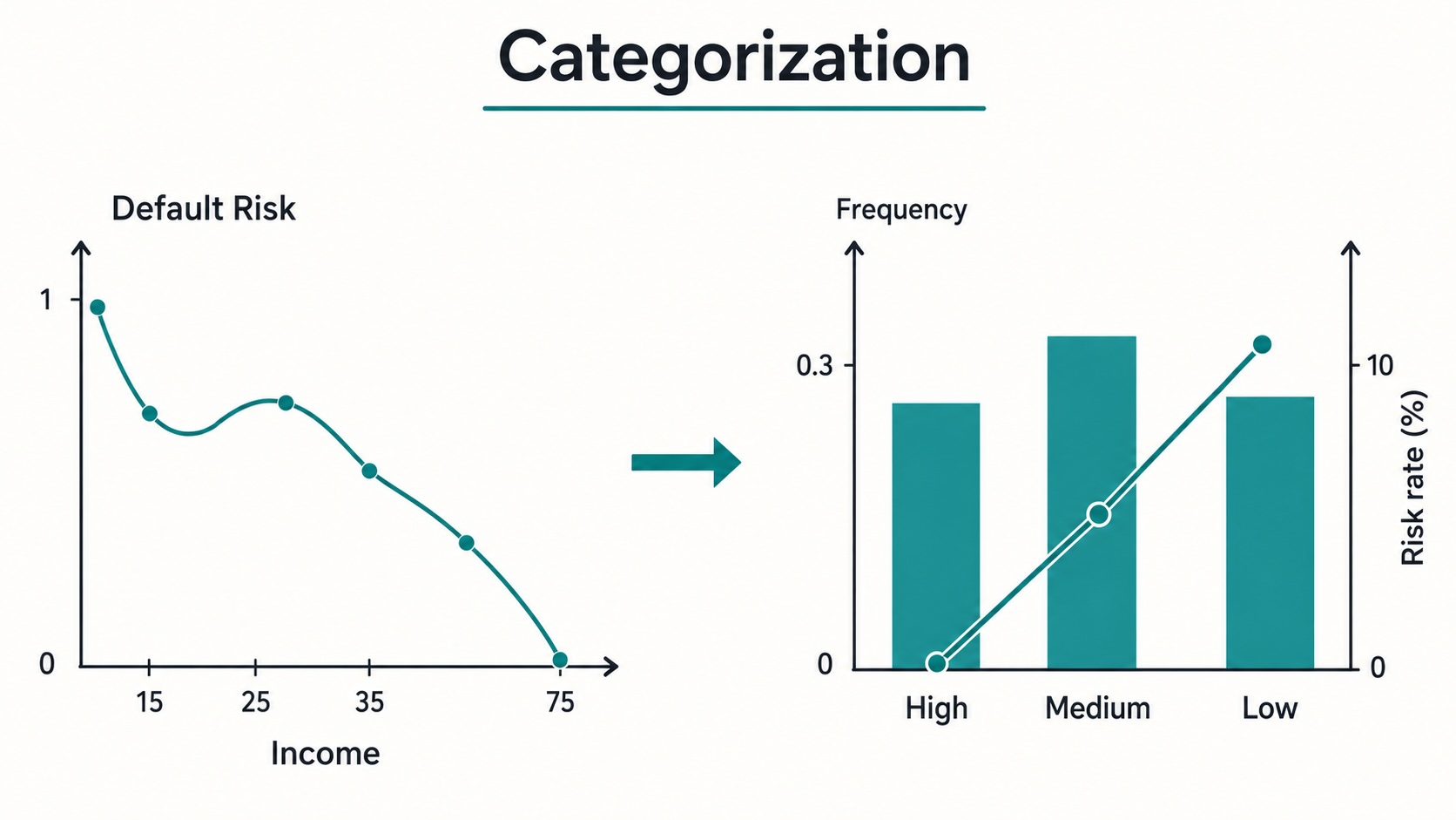
It’s also helpful to visualise, for every class:
- the inhabitants share;
- the default charge.
This may be performed utilizing a mixed bar plot and line plot.

This chart is beneficial as a result of it provides two items of data on the identical time.
The bar plot tells us whether or not the class comprises sufficient observations.
The road plot tells us whether or not the class has a coherent default charge.
An excellent last binning ought to have each a adequate inhabitants dimension and a significant danger sample.
The identical cut-off factors should then be utilized to the check and out-of-time datasets.
This level is essential.
The binning should be outlined on the coaching pattern after which utilized unchanged to validation samples. In any other case, we introduce information leakage and make the validation much less dependable.
Conclusion
On this article, we studied why categorization is a key step in credit score scoring mannequin growth.
Categorization applies to each categorical and steady variables.
For categorical variables, it helps cut back the variety of modalities and makes the mannequin simpler to estimate and interpret.
For steady variables, it helps seize non-linear danger patterns, cut back the affect of outliers, deal with lacking values, enhance stability, and put together variables for Weight of Proof transformation.
We additionally mentioned a number of categorization strategies, together with equal-interval binning, equal-frequency binning, Chi-square-based grouping, and Weight of Proof-based grouping.
In apply, categorization shouldn’t be handled as a mechanical preprocessing step. An excellent categorization should fulfill statistical, enterprise, and stability necessities.
It ought to create courses which are sufficiently populated, clearly ordered when it comes to danger, steady over time, and simple to clarify.
That is particularly essential when the ultimate mannequin is a logistic regression scorecard. In that context, WoE-based categorization helps remodel uncooked variables into steady danger courses which are naturally aligned with the log-odds construction of the mannequin.
The principle takeaway is that this:
A credit score scoring mannequin is barely as dependable because the variables that enter it.
If variables are noisy, unstable, poorly grouped, or troublesome to interpret, even a very good algorithm might produce a weak mannequin.
However when variables are fastidiously categorized, the mannequin turns into extra sturdy, extra interpretable, and simpler to observe in manufacturing.
What about you? In what conditions do you categorize variables, for what causes, and utilizing which strategies?


