From Phrases to Vectors: What Occurs in Between?

We use AI instruments on a regular basis for varied duties like asking a query about one thing or fixing an issue, and we get responses in seconds.

Now have you ever ever questioned about how the machine can perceive our language and reply to our questions? Or, put one other approach, how the machine is processing the language and producing a response?

As people who find themselves interested in studying the newest applied sciences in AI and ML, it is pure to marvel what is going on internally.

We have already got an thought about machine studying fashions, and one factor we all know is that these fashions work with numbers, or numerical representations of the info, as we preprocess the info and feed it into the mannequin and the mannequin learns patterns in that knowledge.

When i began exploring this, i got here throughout ideas like tokenization, embeddings, transformer structure, and so on. However i do not wish to soar into these ideas instantly; as an alternative, let’s construct from the fundamentals in order that it may be simple to grasp the extra superior ideas.

Now the query in entrance of us is to understand how the textual content is transformed to numbers.

One of many basic approaches for doing that is TF-IDF vectorization.

···

You would possibly already find out about this idea or you will have even used it in considered one of your initiatives.

So why do i begin right here?

Right here, i’m constructing in direction of embeddings and different essential ideas in NLP and AI. As an alternative of instantly ranging from ideas like embeddings, i wish to begin with fundamentals and see how we characterize textual content as numbers, one step at a time.

TF-IDF is a basic matter and that i wish to discover it in my approach by beginning with a easy datset and looking out on the math and geometry and see what the outcomes truly characterize.

In the event you’re already accustomed to TF-IDF, you need to use this text as a fast refresher or skip forward to the upcoming embeddings articles if that is what you are interested in.

However for those who’re new to textual content illustration, let’s begin from the start and see what occurs when phrases turn into numbers.

···

···

What Is TF-IDF?

It is time to study what TF-IDF truly is and what it does.

TF-IDF stands for Time period Frequency–Inverse Doc Frequency.

It combines two concepts.

One is Time period Frequency, which suggests ‘How usually does a phrase seem in a specific doc’ and the second is Inverse Doc Frequency which suggests ‘How frequent or uncommon is that phrase throughout all paperwork?’

After calculating TF and IDF, we multiply them.

TF-IDF=TF×IDF​.

Let’s examine how we calculate this intimately.

···

Let’s Begin With a Easy Dataset

For that permit’s think about a easy dataset.

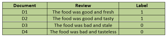
We could have any objective with this dataset, like performing classification, discovering comparable paperwork, or data retrieval, however we first must characterize these in a numerical kind so {that a} machine studying mannequin can course of additional.

Step 1: Tokenization

Step one we have to do is to interrupt every evaluation into particular person phrases.

That is referred to as tokenization.

We do that as a result of TF-IDF works by taking a look at particular person phrases and the way essential they’re inside every doc and throughout all of the paperwork.

D1 : [“the”, “food”, “was”, “good”, “and”, “fresh”]

D2 : [“the”, “food”, “was”, “good”, “and”, “tasty”]

D3 : [“the”, “food”, “was”, “bad”, “and”, “stale”]

D4 : [“the”, “food”, “was”, “bad”, “and”, “tasteless”]

That is what we get after tokenization, and every phrase is known as token.

···

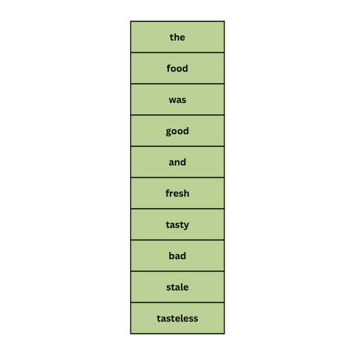
Step 2: Constructing the Vocabulary

The following step is to create a vocabulary which is the gathering of all of the distinctive values throughout all of the paperwork we now have within the dataset.

For our knowledge, the vocabulary we now have is:

···

Step 3: Time period Frequency (TF)

Now we calculate the time period frequency or just we name it as TF.

That is the primary a part of TF-IDF.

We calculate the time period frequency utilizing:

Right here, ‘t’ represents a time period(phrase) and ‘d’ represents the doc(evaluation).

Now let’s think about D1, after tokenization we now have: [“the”, “food”, “was”, “good”, “and”, “fresh”].

Contemplate the phrase ‘meals’, which seems solely as soon as within the doc.

Subsequently, the time period frequency of ‘meals’ is 1/6.

Each phrase seems solely as soon as in D1, which suggests the time period frequency right here is similar for all of the phrases.

Now if we have a look at our vocabulary, it comprises all of the distinctive phrases from all 4 paperwork, not simply the phrases in D1.

So, once we create the numerical illustration for D1, we have to have a price for each phrase on this vocabulary.

For instance, think about the phrase ‘tasty’, it does not seem in D1.

The TF of ‘tasty’ in D1 is zero.

The identical factor can be utilized to the opposite phrases which aren’t in D1.

So, within the order of our vocabulary, the TF values of D1 are:

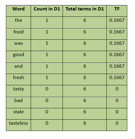
In the identical approach, we get TF values for all of the phrases throughout all paperwork.

···

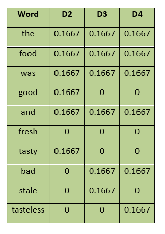
Now we now have calculated the Time period Frequency for all of the 4 paperwork.

We noticed that the TF worth relies upon solely on how usually a phrase seems inside a specific doc.

However TF alone just isn’t sufficient.

For instance, think about the phrases ‘the’ and ‘contemporary’ in D1.

Each phrases seem solely as soon as in D1, however ‘the’ seems in all of the 4 paperwork.

What we will observe right here?

We will say that TF alone can not inform us that the phrase ‘contemporary’ is extra informative for distinguishing D1 from the opposite paperwork.

So, we want one other measure that considers all of the paperwork.

This brings us to IDF which is Inverse Doc Frequency.

···

Step 4: Doc Frequency (DF)

Earlier than continuing with IDF, let’s first perceive the Doc Frequency.

Doc Frequency tells us in what number of paperwork the actual phrase seems.

We should observe that we’re counting paperwork, not the whole variety of instances a phrase seems.

For instance, think about ‘the’: It seems in all of the 4 paperwork.

Subsequently, the doc frequency for ‘the’ is:

We will discover this for each phrase within the vocabulary.

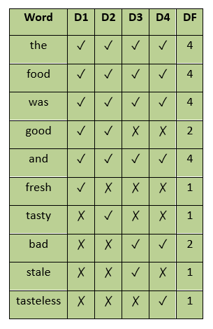
Now we now have the DF for each phrase in our vocabulary. However what can we do with it?

If we observe the DF values, we will see that some phrases have a excessive DF, whereas others have a low DF.

We will sense that phrases with a low DF might be extra important when distinguishing a specific doc from the others.

So, we want a measure that offers greater weight to phrases with low DF and decrease weight to phrases with excessive DF.

That is the place the Inverse Doc Frequency(IDF) is available in.

Right here, we’re utilizing IDF as a result of we would like the burden of the phrase to maneuver in wrong way to DF, which suggests greater DF offers decrease weight, whereas decrease DF offers greater weight.

···

Step 5: Inverse Doc Frequency (IDF)

Now it is time to calculate the IDF values for our vocabulary.

The method we use is:

Right here:

N is the whole variety of paperwork, and DF(t) is the variety of paperwork containing the time period t.

Right here, we use the logarithm to compress the vary of IDF values, in order that very uncommon phrases don’t obtain disproportionately giant weights.

In our dataset, we now have 4 paperwork.

Now we once more think about the phrase ‘the’:

From the Doc Frequency desk, we now have:

Substituting the values into method, we get:

The IDF worth for ‘the’ is 0.

Now, let’s think about one other phrase ‘good’, we get:

We will observe that the IDF worth of ‘good’ is greater than ‘the’, as a result of ‘good’ seems in fewer paperwork.

Utilizing the identical course of, we will calculate the IDF values for each phrase within the vocabulary.

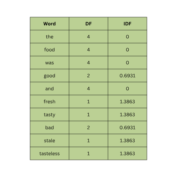
From the above desk, we will observe that:

The phrases ‘the’, ‘meals’, ‘was’ and ‘and’ seem in all 4 paperwork, so their IDF is 0.

The phrases ‘good’ and ‘dangerous’ seem in two paperwork, so their IDF is roughly 0.6931.

The phrases ‘contemporary’, ‘tasty’, ‘stale’ and ‘tasteless’ seem in just one doc, so that they have the very best IDF worth in our dataset, roughly 1.3863.

At this level, we now have each items we want:

One is TF which tells us how often a phrase seems in a specific doc and

the second is IDF which tells us how frequent or uncommon that phrase is throughout the gathering of paperwork.

···

Step 6: Calculating TF-IDF

The following step is to mix these two values to acquire the precise TF-IDF rating for every phrase. We do that by multiplying TF and IDF.

Now, let’s think about our first doc D1:

‘The meals was good and contemporary’

From the sooner calculations, we now have

TF(the,D1)=0.1667 and IDF(the)=0.

Subsequently:

The TF-IDF rating for ‘the’ is zero, this occurred as a result of it seems in each doc. It is TF tells us it seems in D1 nevertheless it’s IDF tells us that it’s common throughout all paperwork.

Let’s apply the identical thought to ‘good’.

We already know:

TF(good,D1)=0.1667 and IDF(good)=0.6931

This manner we calculate the TF-IDF scores for all of the phrases in D1.

···

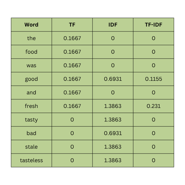
From TF-IDF Scores to Vectors

We now have the TF-IDF scores for each phrase in D1.

The order of our vocabulary is:

[the, food, was, good, and, fresh, tasty, bad, stale, tasteless]

Now, we will write the TF-IDF illustration of D1 as:

First we now have the evaluation D1 as textual content, however now we represented it utilizing numbers.

We will observe that the numbers are in a set order, with every quantity representing a phrase from our vocabulary.

The primary quantity represents the, the second represents meals, the fourth represents good, and so forth.

Because it has ordered assortment of numerical values, we will characterize it as a vector.

In our vocabulary, we now have 10 phrases, so right here we now have a 10-dimensional vector, the place every dimensions corresponds to at least one phrase within the vocabulary.

In the identical approach, we get the TF-IDF representations for the opposite paperwork.

We now have an thought of the mathematics behind TF-IDF.

···

Implementing TF-IDF in Python

However in real-world functions, we use Python and libraries reminiscent of scikit-learn to calculate the values.

Let’s take a look at how it’s carried out in python.

Code:

from sklearn.feature_extraction.textual content import TfidfVectorizer# Our evaluationsevaluations = [    "The food was good and fresh",    "The food was good and tasty",    "The food was bad and stale",    "The food was bad and tasteless"]# Create the TF-IDF vectorizervectorizer = TfidfVectorizer()# Convert the evaluations into TF-IDF vectorsX = vectorizer.fit_transform(evaluations)# Get the vocabulary/optionsprint("Vocabulary:")print(vectorizer.get_feature_names_out())# Show the TF-IDF matrixprint("nTF-IDF Matrix:")print(X.toarray())# Show the form of the matrixprint("nShape:")print(X.form)

Output:

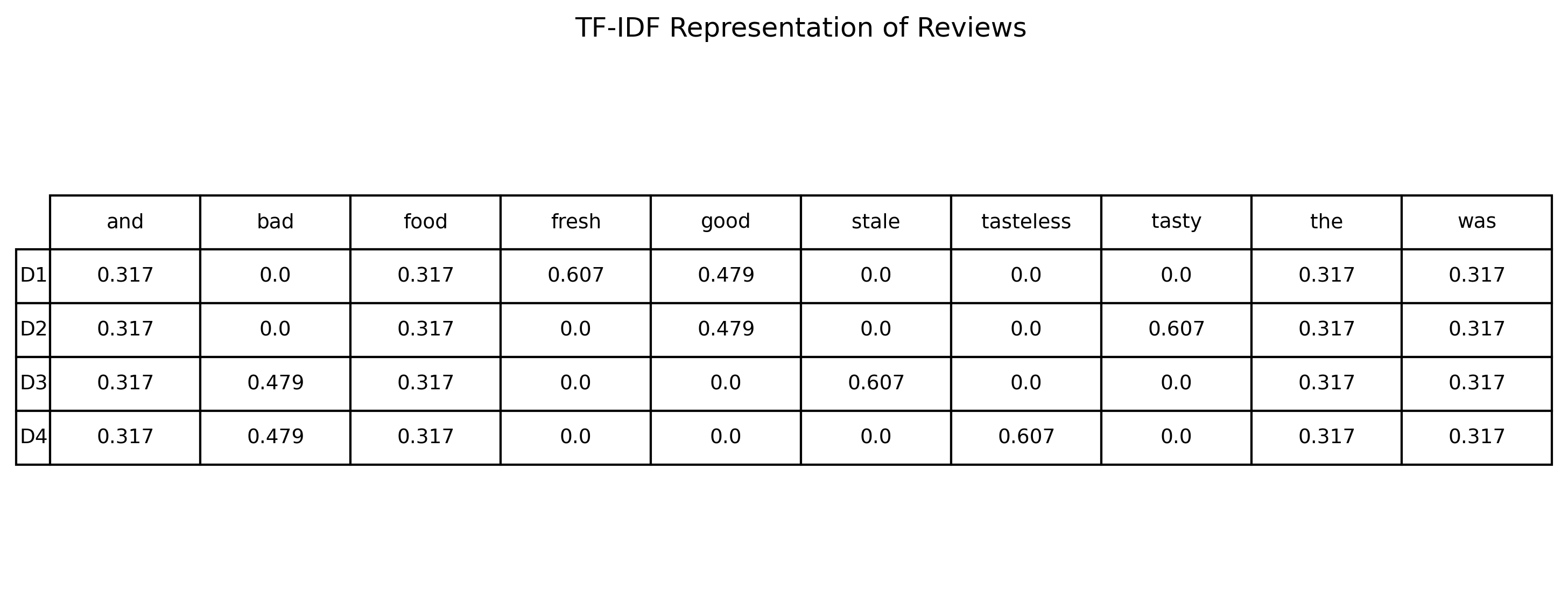
Why Are the Python Values Completely different?

We will observe that the values we bought through the use of python are completely different from what we bought by handbook calculation.

This occurs as a result of TF-IDF makes use of a smoothed IDF method.

The opposite factor is that TF-IDF vectorizer additionally normalizes every doc vector, which ends up in scaling the values in a vector based mostly on the general size of that vector.

However why that is finished in python implementation.

It’s as a result of smoothing is used to vary the conduct of IDF at boundary circumstances, for instance think about phrase ‘the’ in our vocabulary, it is IDF worth is 0 however once we use the smoothed method it turns into 1.

The python implementations reminiscent of scikit-learn use these strategies to maintain the IDF calculation in a constant kind.

Whereas normalization reduces the affect of doc size on the magnitude of the TF-IDF vector.

For instance, an extended doc will produce a larger-magnitude vector just because it comprises extra phrases. Normalization scales the vector, permitting us to focus extra on the sample of TF-IDF values moderately than the general measurement of the vector.

···

Visualizing TF-IDF Vectors With PCA

Now we now have 4 10-dimensional vectors.

We wish to visualize them, however we can not instantly plot a 10-dimensional vector house on a 2D graph.

What we will do is, use a dimensionality discount method to scale back the variety of dimensions and visualize the ensuing representations in a 2D plot.

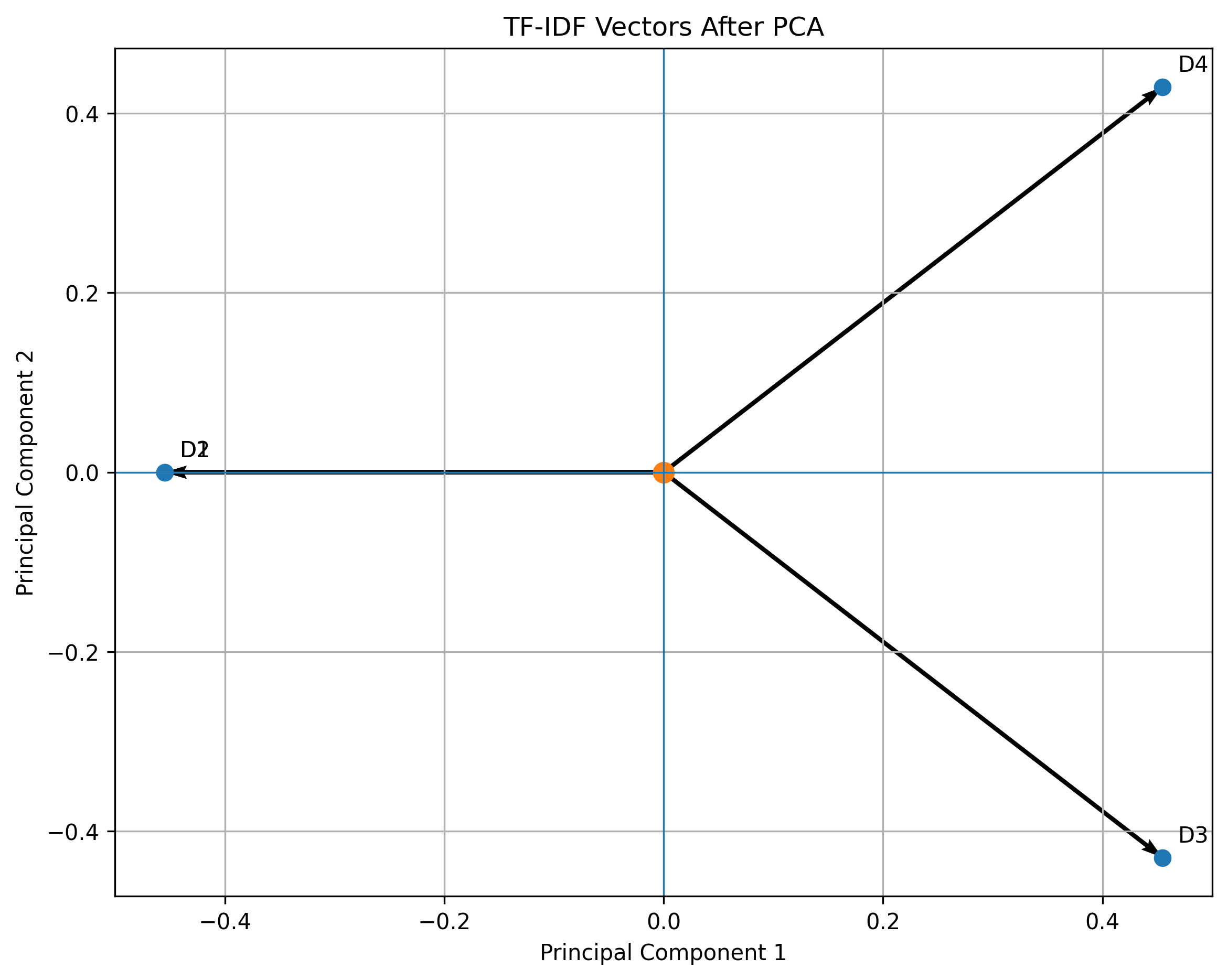
Earlier than making use of PCA, every evaluation was represented by 10 TF-IDF values and after making use of PCA, every evaluation is represented by simply two values, which we will name as a 2nd-vector.

On this 2D PCA projection, paperwork with comparable numerical representations have a tendency to look nearer collectively.

We are going to focus on about each dimensionality discount method intimately within the upcoming articles.

···

Utilizing TF-IDF for Textual content Classification

We now transformed our evaluations to the numerical representations, however this isn’t our closing objective.

Our closing objective is to make use of this numerical representations to carry out an actual world activity like classification.

In the event you bear in mind, our dataset has labels ‘1’ and ‘0’.

‘1’ means optimistic and ‘0’ means adverse.

Now we will use these numerical representations as our enter options and labels because the goal for a machine studying mannequin.

For instance, let’s use the logistic regression for classification.

For classification, we are going to use the TF-IDF illustration from our Python implementation, not the 2D illustration produced by PCA.

First, let’s have a look at how our dataset now seems:

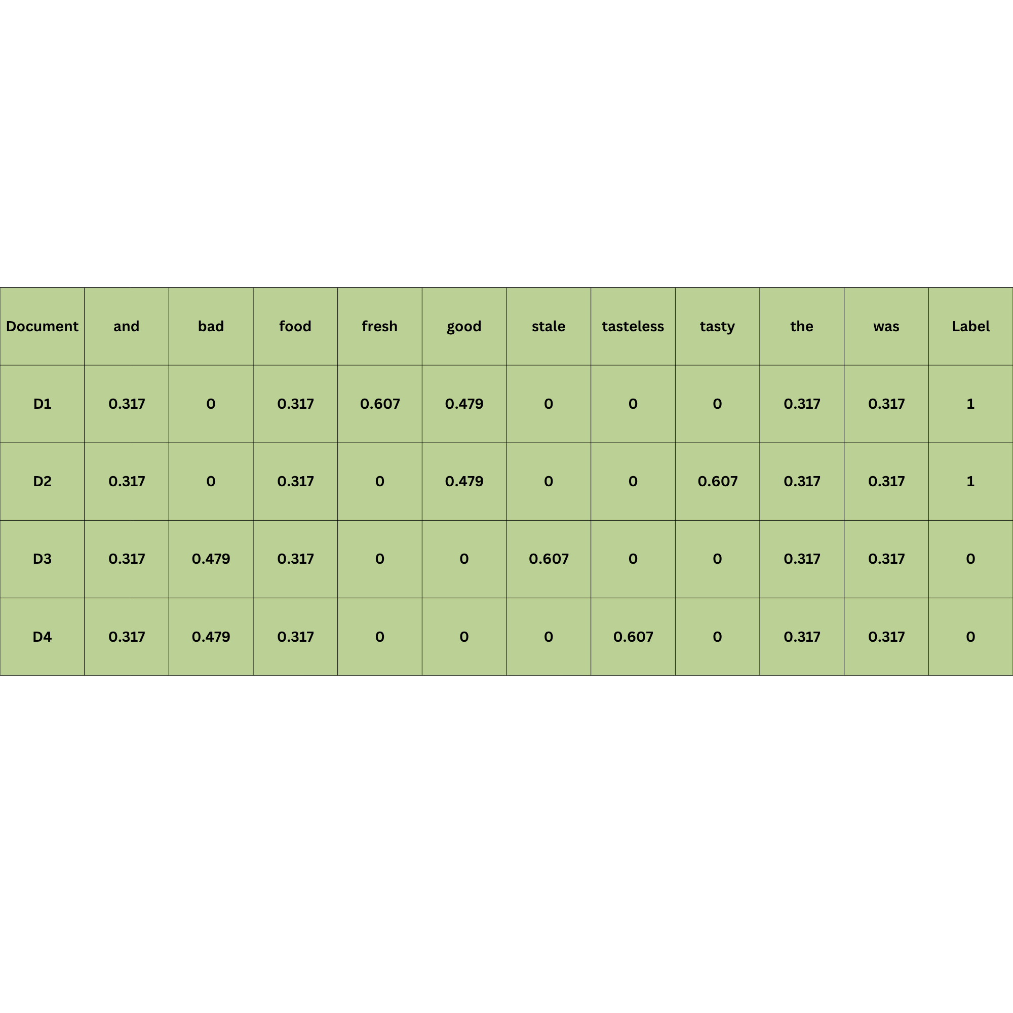
Our dataset is not made up of textual content. We have now remodeled it right into a numerical machine studying dataset. Every phrase within the vocabulary is a characteristic.

Now let’s use Python to implement the logistic regression to foretell the label.

Everyone knows that logistic regression learns a weight for every characteristic and in addition learns a bias.

The mannequin first calculates a rating:

Later we use the sigmoid perform to get the worth that may be interpreted as a likelihood between 0 and 1.

Now let us take a look at the code.

from sklearn.feature_extraction.textual content import TfidfVectorizerfrom sklearn.linear_model import LogisticRegression# Our datasetevaluations = [    "The food was good and fresh",    "The food was good and tasty",    "The food was bad and stale",    "The food was bad and tasteless"]# Goal Labelslabels = [1, 1, 0, 0]# Convert textual content into TF-IDF optionsvectorizer = TfidfVectorizer()X = vectorizer.fit_transform(evaluations)# Create and practice the Logistic Regression mannequinmannequin = LogisticRegression()mannequin.match(X, labels)# Show the discovered weightsfeature_names = vectorizer.get_feature_names_out()print("Discovered weights:")for phrase, weight in zip(feature_names, mannequin.coef_[0]):    print(f"{phrase}: {weight:.4f}")# Show the discovered biasprint("nBias:", mannequin.intercept_[0])# Predict the coaching examplespredictions = mannequin.predict(X)print("nPredictions:", predictions)# Predict for a brand new evaluationnew_review = ["The food was fresh"]new_vector = vectorizer.rework(new_review)print("nPrediction likelihood:")print(mannequin.predict_proba(new_vector))print("nPredicted class:")print(mannequin.predict(new_vector))

Output:

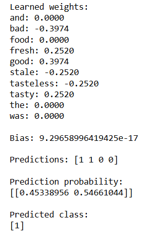
We have now now skilled the Logistic Regression mannequin and used it to foretell the label for a brand new evaluation.

Right here, we will observe that the phrases within the new evaluation are already current in our vocabulary. We then transformed the brand new evaluation right into a TF-IDF vector utilizing the similar fitted vectorizer that we used for the coaching knowledge.

···

What Occurs When We Encounter a New Phrase?

For instance, we now have a brand new evaluation: ‘the meals was scrumptious’.

The phrase ‘scrumptious’ just isn’t current in our vocabulary. The mannequin has no discovered characteristic or weight for “scrumptious.”

Let’s predict the label for this evaluation.

Code:

new_review = ["The food was delicious"]new_vector = vectorizer.rework(new_review)print("TF-IDF vector:")print(new_vector.toarray())print("Prediction:")print(mannequin.predict(new_vector))print("Prediction likelihood:")print(mannequin.predict_proba(new_vector))

Output:

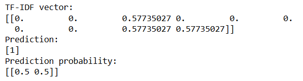
From the output, we will observe one thing attention-grabbing. Because the phrase ‘scrumptious’ just isn’t in vocabulary, it doesn’t contribute any characteristic to the TF-IDF vector. So the mannequin makes its prediction utilizing solely the opposite three phrases which it is aware of already.

We will additionally see that the prediction likelihood is 50% for every class. This implies the mannequin doesn’t have sufficient data from the out there options to obviously distinguish between the 2 courses for this evaluation.

Let’s examine what truly occurred with our new evaluation “the meals was scrumptious”.

The fitted vectorizer checks every phrase towards the vocabulary it discovered from the coaching knowledge. It makes use of the IDF values already discovered from the coaching knowledge.

The phrases “the,” “meals,” and “was” are current within the vocabulary, whereas “scrumptious” just isn’t. Subsequently, no characteristic is created for “scrumptious,” and its contribution to the vector is 0.

The three identified phrases obtain TF-IDF values, leading to roughly 0.577 for every of them. This provides us the vector proven beneath.

[0. 0. 0.577 0. 0. 0. 0. 0. 0.577 0.577]

···

Limitations of TF-IDF

What we will perceive from this?

We will observe a limitation of TF-IDF, the place a phrase that was not current within the coaching vocabulary can not contribute to the mannequin’s prediction.

There’s additionally one other limitation, even when phrases are current in vocabulary, it treats them as separate options.

For instance, if we now have phrases ‘good’ and ‘wonderful’ in our vocabulary, they’re represented as two completely different phrases, with none inherent understanding that they’ve comparable meanings.

That does not imply we do not use TF-IDF in any respect. It’s nonetheless utilized in duties like textual content classification, spam detection and so on.

···

From TF-IDF to Embeddings

Now the query is as an alternative of representing a phrase merely as a characteristic with a TF-IDF rating, can we characterize a phrase utilizing numbers that seize its relationships with different phrases?

That is the place embeddings are available.

They’re extensively utilized in functions reminiscent of semantic search, query answering, advice methods, retrieval augmented era (RAG) and so on.

···

I hope you discovered this weblog helpful for understanding the fundamentals on how textual content might be transformed right into a numerical illustration.

In the event you suppose one thing is lacking or might be improved, be happy to depart a touch upon Linkedin.

Within the subsequent article, we’ll begin from the fundamentals and discover how embeddings characterize phrases as vectors.

By the way in which, if you have not learn my latest weblog on sigmoid perform, you’ll be able to learn it right here.

Thanks for studying!