


Rework boring default Matplotlib line charts into gorgeous, personalized visualizations

Everybody who has used Matplotlib is aware of how ugly the default charts appear to be. On this sequence of posts, I’ll share some methods to make your visualizations stand out and replicate your particular person model.
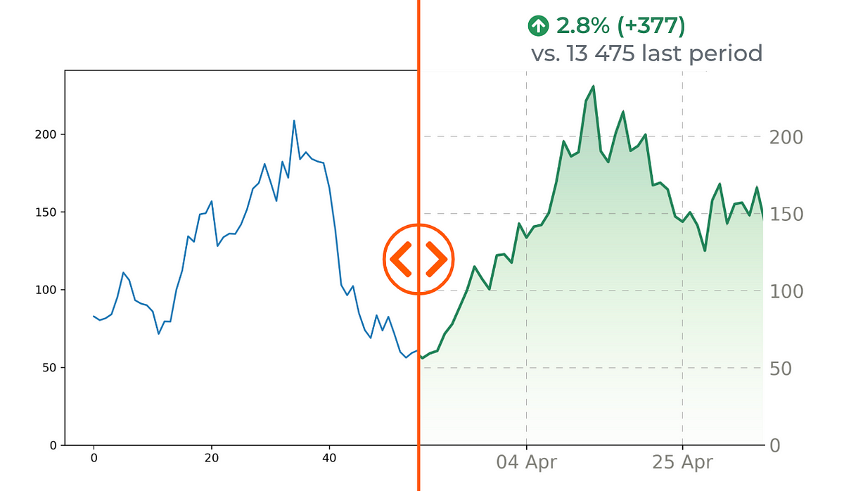
We’ll begin with a easy line chart, which is broadly used. The principle spotlight will likely be including a gradient fill beneath the plot — a activity that’s not fully easy.
So, let’s dive in and stroll by means of all the important thing steps of this transformation!
Let’s make all the mandatory imports first.
import pandas as pd
import numpy as np
import matplotlib.dates as mdates
import matplotlib.pyplot as plt
import matplotlib.ticker as ticker
from matplotlib import rcParams
from matplotlib.path import Path
from matplotlib.patches import PathPatchnp.random.seed(38)
Now we have to generate pattern knowledge for our visualization. We’ll create one thing much like what inventory costs appear to be.
dates = pd.date_range(begin='2024-02-01', durations=100, freq='D')
initial_rate = 75
drift = 0.003
volatility = 0.1
returns = np.random.regular(drift, volatility, len(dates))
charges = initial_rate * np.cumprod(1 + returns)x, y = dates, charges
Let’s examine the way it appears to be like with the default Matplotlib settings.
repair, ax = plt.subplots(figsize=(8, 4))
ax.plot(dates, charges)
ax.xaxis.set_major_locator(mdates.DayLocator(interval=30))
plt.present()

Not likely fascination, proper? However we are going to steadily make it trying higher.
- set the title
- set common chart parameters — measurement and font
- putting the Y ticks to the suitable
- altering the primary line coloration, model and width
# Common parameters
fig, ax = plt.subplots(figsize=(10, 6))
plt.title("Day by day guests", fontsize=18, coloration="black")
rcParams['font.family'] = 'DejaVu Sans'
rcParams['font.size'] = 14# Axis Y to the suitable
ax.yaxis.tick_right()
ax.yaxis.set_label_position("proper")
# Plotting primary line
ax.plot(dates, charges, coloration='#268358', linewidth=2)

Alright, now it appears to be like a bit cleaner.
Now we’d like so as to add minimalistic grid to the background, take away borders for a cleaner look and take away ticks from the Y axis.
# Grid
ax.grid(coloration="grey", linestyle=(0, (10, 10)), linewidth=0.5, alpha=0.6)
ax.tick_params(axis="x", colours="black")
ax.tick_params(axis="y", left=False, labelleft=False) # Borders
ax.spines["top"].set_visible(False)
ax.spines['right'].set_visible(False)
ax.spines["bottom"].set_color("black")
ax.spines['left'].set_color('white')
ax.spines['left'].set_linewidth(1)
# Take away ticks from axis Y
ax.tick_params(axis='y', size=0)

Now we’re including a tine esthetic element — yr close to the primary tick on the axis X. Additionally we make the font coloration of tick labels extra pale.
# Add yr to the primary date on the axis
def custom_date_formatter(t, pos, dates, x_interval):
date = dates[pos*x_interval]
if pos == 0:
return date.strftime('%d %b '%y')
else:
return date.strftime('%d %b')
ax.xaxis.set_major_formatter(ticker.FuncFormatter((lambda x, pos: custom_date_formatter(x, pos, dates=dates, x_interval=x_interval))))# Ticks label coloration
[t.set_color('#808079') for t in ax.yaxis.get_ticklabels()]
[t.set_color('#808079') for t in ax.xaxis.get_ticklabels()]

And we’re getting nearer to the trickiest second — find out how to create a gradient underneath the curve. Really there is no such thing as a such choice in Matplotlib, however we will simulate it making a gradient picture after which clipping it with the chart.
# Gradient
numeric_x = np.array([i for i in range(len(x))])
numeric_x_patch = np.append(numeric_x, max(numeric_x))
numeric_x_patch = np.append(numeric_x_patch[0], numeric_x_patch)
y_patch = np.append(y, 0)
y_patch = np.append(0, y_patch)path = Path(np.array([numeric_x_patch, y_patch]).transpose())
patch = PathPatch(path, facecolor='none')
plt.gca().add_patch(patch)
ax.imshow(numeric_x.reshape(len(numeric_x), 1), interpolation="bicubic",
cmap=plt.cm.Greens,
origin='decrease',
alpha=0.3,
extent=[min(numeric_x), max(numeric_x), min(y_patch), max(y_patch) * 1.2],
side="auto", clip_path=patch, clip_on=True)

Now it appears to be like clear and good. We simply want so as to add a number of particulars utilizing any editor (I want Google Slides) — title, spherical border corners and a few numeric indicators.

The complete code to breed the visualization is beneath:


