Binning or Characteristic Choice: Which One Gained Us an Insurance coverage Hackathon?

Zacharie Buisson co-built the profitable answer with me. Each quantity beneath is measured, and each pocket book is saved with the outputs that produced it.

Disclosure: I’m the creator and maintainer of AutoCarver, an open-source (MIT) library. Learn the library sections with that in thoughts. Each quantity will be checked from the repository and datasets linked beneath. All photos are by the creator, generated from the problem information (Etalab Licence Ouverte 2.0).

···

The end line, first

In 2025, we took first place in an insurance coverage hackathon. A yr later, we audited that outcome, and the audit reversed the assumption beneath it. Binning did beat not binning. Nevertheless, our personal library’s bins had been indistinguishable from a rival’s. The one achieve that was not an in depth name was velocity: 126 minutes of carving went all the way down to 4.3, on the identical options.

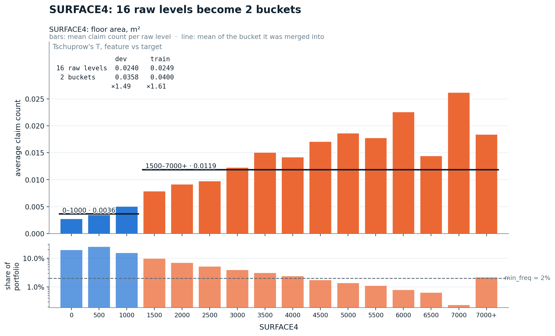
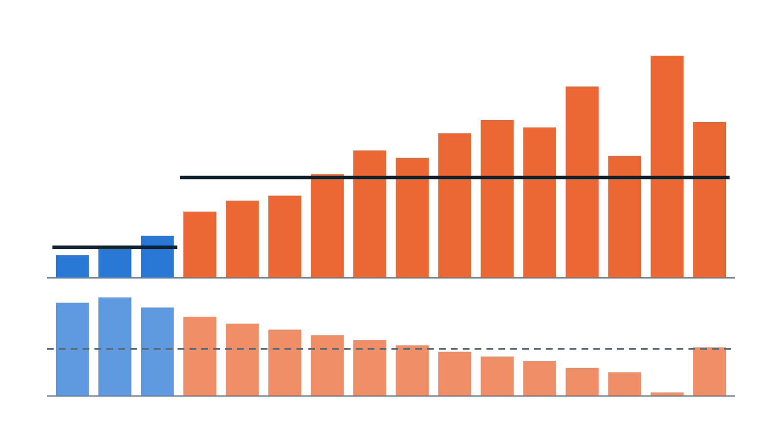
The determine reveals one actual function from the problem information. The insurance policies are anonymised French farms, priced towards fireplace. Ground space is available in sixteen bands, and declare frequency climbs roughly tenfold throughout them. Supervised binning cuts these bands in two, at 1000 m². Finer choices existed, since ten of the bands clear the two% min_freq ground. Nevertheless, the carver’s affiliation measure ranked this lower above all of them (instruments/make_hero_chart.py --explain). The decrease panel explains the selection. Each band from 4500 m² to 7000 m² covers underneath 2% of the portfolio, so essentially the most dramatic charges relaxation on a handful of insurance policies. With out supervised binning, a pipeline would maintain all sixteen bands, or merge them by hand. We carved 400 options this fashion, and we believed it was half of why we gained.

This method took us to first place within the Crédit Agricole Assurances Information Science Academy hackathon [5], out of greater than 500 contributors. The hackathon was ranked on the non-public leaderboard of the general public ENS Problem Information #161 [1], because it stood when the hackathon closed in spring 2025. The problem remains to be open, so the stay leaderboard has moved on since. Because of this, no quantity on this article is a leaderboard rating. The problem additionally served because the working instance within the Information Science course we taught at CY Tech.

We re-ran the pipeline with the present model of the library to examine two issues: whether or not it was sooner, and whether or not it was extra correct. Velocity was straightforward to measure. Accuracy took three experiments. Yearly-on-year accuracy achieve turned out smaller than the noise in our personal tuning, and the sting we had credited to carving got here from which options the selector saved. To point out this, we ran 4 seeds per arm, measured each margin towards its personal unfold, and held one function set fixed to separate two steps we had all the time run collectively.

1. The issue

For a farm, a single fireplace can destroy barns, equipment and inventory, and this danger is rising. The IPCC assesses that fireplace hazard circumstances rose throughout Europe from 1980 to 2019, with substantive will increase in Western and Central Europe (excessive confidence). It additionally assesses that wildfire danger can rise in each European area between 1.5 °C and three °C of warming (medium to excessive confidence) [6]. Insurers see the identical pattern. Swiss Re places 2025 insured natural-catastrophe losses at USD 107 bn, and calls wildfire the fastest-growing line, at close to 12% a yr [7].

In France, Crédit Agricole Assurances covers this danger for farms via Pacifica, its property-and-casualty service, which writes the Contrat Multirisque Agricole. Problem #161, referred to as AssurPrime, asks contributors to cost the fireplace cowl of this contract from anonymised coverage information. Hearth is a big share of the contract’s claims [1]. Our work makes use of a single snapshot of this information and no temporal evaluation, so not one of the local weather developments above is a discovering of our mannequin.

The problem scores CHARGE, the entire declare price of a coverage. Insurers don’t predict such a value in a single step. As actuaries have carried out for many years, they issue it:

CHARGE is strictly this product, scaled by the coverage’s years of publicity, and the problem information offers each components. Two issues make the issue tougher than it appears to be like. First, claims are uncommon. Virtually each coverage has zero claims, so a mannequin that predicts zero for everybody appears to be like correct however is ineffective. Second, the 2 targets behave very in another way. Frequency is a small depend, whereas severity is a heavy-tailed quantity, and a single mannequin for each would blur every of them. We subsequently constructed two fashions.

2. The profitable recipe (2025)

Our 2025 answer used neither a large mannequin nor an ensemble of ensembles. It rested on three choices. First, we factored the issue into frequency × severity, as actuaries do. Second, we binned each function towards the goal with AutoCarver, the open-source library named within the disclosure [2]. Third, we weighted the uncommon sign. The audit on this article solely checks the second choice.

2.1 Carving the options first

In addition to the anonymised coverage options, we joined a wildfire-exposure profile for every geographic zone, constructed from BDIFF, France’s nationwide forest-fire database [3]: burnt space, fireplace counts by trigger, variety of fireplace stations and wind zone (23,462 fires recorded over 2016–2023).

Uncooked insurance coverage options are messy: high-cardinality categoricals, ordinal ranges with tiny populations, skewed numerics, and NaNs that carry that means. Given such options, a tree mannequin spends its depth rediscovering construction that would have been handed to it.

Supervised binning offers that construction. For every function, AutoCarver searches for the admissible grouping with the strongest statistical affiliation with the goal. A grouping is admissible underneath three constraints: a minimal bin frequency, a most variety of bins per function, and validation on a held-out dev set. The final constraint issues most, since a grouping that solely works on the coaching information is rejected. In observe, the function varieties are declared as soon as and the whole lot is carved in a single match:

# AutoCarver 7.0.5, as written in 2025. The present API seems later.from AutoCarver import Options, MulticlassCarveroptions = Options(    categoricals=["property_type", "region", ...],    quantitatives=["insured_value", "surface", ...],    ordinals={"quality_band": ["low", "mid", "high", "premium"]},)carver = MulticlassCarver(options=options, min_freq=0.02, max_n_mod=5)train_carved = carver.fit_transform(prepare, prepare["n_claims"], X_dev=dev, y_dev=dev["n_claims"])carver.abstract  # each bucket: frequency, goal fee, affiliation

Notice that this snippet nonetheless runs at present, nevertheless it does one thing else. In 7.0.5, MulticlassCarver carved one-vs-rest, so each uncooked function got here again as a number of columns. That behaviour is now referred to as OneVsRestCarver.

The plain different is optbinning [4]. The place AutoCarver searches groupings heuristically, optbinning states the merge of CART prebins as a CP/MILP drawback and solves it precisely, inside a time restrict. We selected in another way for 3 causes, which concern our setting fairly than the library itself. First, we needed each grouping examined on a held-out pattern, and match(x, y) has no notion of 1. Second, our goal is ordered, and MulticlassOptimalBinning doesn’t deal with it as such. Third, its multiclass path handles numerical options solely, whereas most of our 435 options are categorical or declared ordinals. On the time, these had been solely causes. We measure their penalties additional beneath.

With binning, ordinals had been merged of their pure order, and one pipeline dealt with all function varieties. Lacking values are by no means silently imputed: with dropna=True, AutoCarver carves NaN as its personal bucket. We selected dropna=False as a substitute, and let XGBoost route them natively. After carving, ClassificationSelector pre-selected options by affiliation and pruned redundant ones in a single go.

2.2 Frequency: a weighted multiclass mannequin

Virtually no coverage has greater than two claims, so we handled frequency as a multiclass drawback over 0 / 1 / 2+. Inverse-frequency class weights stopped the mannequin from collapsing onto the bulk class. The legislation of whole expectation then turns the category chances again into an anticipated frequency:

Each log loss on this article is the class-weighted one, with those self same inverse-frequency weights, since that is what the search minimised. For reference, a relentless base-rate mannequin scores 0.041 unweighted and 4.47 weighted. A uniform guess of ⅓ per class scores 1.099. Our fashions rating round 0.92.

2.3 Severity and tuning

The severity mannequin solely sees insurance policies with claims. The trick we credit score most is to weight every statement by the frequency mannequin’s absolute error. The severity mannequin then concentrates on the insurance policies the place the primary stage was incorrect. This works as an affordable, boosting-like correction throughout the 2 phases. We measured its impact in the course of the competitors, on the general public leaderboard, however that comparability just isn’t reproduced on this article. Each fashions are XGBoost, tuned with Optuna. One thought from the tuning is value reusing: the variety of pruned options was itself a hyper-parameter.

3. What a yr of releases really purchased

We gained with AutoCarver 7.0.5. A yr later, we re-ran each pipelines on the present model, with the identical information, the identical prepare/dev cut up and the identical XGBoost search funds. Each step is seeded, so the 2026 numbers beneath will be reproduced precisely (see Setup).

The Setup part lists what else modified between the 2 variations. The principle level is that solely the 2026 aspect is seeded, so the velocity comparisons are clear, however the metric comparisons aren’t.

3.1 Multiprocessing: the gradual step received quick

Carving the 680 MB of coaching information was the slowest step of our 2025 loop.

# AutoCarver 7.7.3from AutoCarver import OrdinalCarverfrom AutoCarver.discretizers import ProcessingConfigcarver = OrdinalCarver(options=options, min_freq=0.02, max_n_mod=5, config=ProcessingConfig(n_jobs=6))

The desk provides the carving wall-clock time on the total dataset (383,610 rows, ~435 qualitative options, one machine, runs serialised):

Model 7.0.5 ran in a single course of, whereas at present’s carve ran on 6 employees, so good scaling alone provides 6×. The remaining issue, ~4× on the frequency carve and ~5.6× on severity, comes from the dynamic-programming top-k search that changed brute-force enumeration. The 2026 severity carve additionally ran at a decrease min_freq (0.02 towards 0.03), so 33.8× is conservative. Not like the accuracy outcomes in a while, these good points aren’t shut calls. The identical carve has come again at 120.0, 126.8 and 129.4 s on this machine, a selection of seven.8%, nowhere close to the 24× hole.

3.2 An ordinal goal

Our claim-count goal just isn’t solely multiclass. It’s ordered (0 < 1 < 2+), and the 2025 MulticlassCarver ignored that order. OrdinalCarver optimises the bins towards an ordinal goal utilizing Kendall’s tau-c. We scored the carvings on a typical yardstick, tau-c on the dev set. OrdinalCarver matches the affiliation per function of the 2025 one-vs-rest geometry, with 2.07× fewer columns and a pair of.05× fewer buckets, in a carve 3.8× sooner. We additionally in contrast it with the unordered multiclass carving, which differs solely in whether or not the order is used. The 2 return an identical bucketings on 210 of 364 options, and the ordinal one wins 111 to 43 on the remaining (two-sided signal check, p ≈ 4×10⁻⁸). The route is dependable, however the measurement is small: +0.000107 in imply tau-c. Declaring ordinal options is subsequently definitely worth the effort. Nevertheless, none of those carvings was carried via choice and tuning, so we declare no impact on the ultimate metric.

3.3 Did the brand new model win by extra?

The desk beneath compares the 2 pipelines finish to finish.

The frequency row of this desk just isn’t a outcome, and it took a devoted experiment to seek out this out. The 2 frequency numbers differ by 0.00055. The 2026 quantity comes from a seeded search that reproduces to sixteen vital figures, so it’s tempting to learn the hole as actual. To examine it, we re-ran the an identical function units underneath 4 TPE seeds, altering nothing else:

Throughout the 4 seeds, the frequency log loss spreads over 0.0101. That is eighteen instances the hole we had been about to interpret. Three seeds land above the 2025 baseline and one lands beneath it, so the signal of the comparability will depend on the seed. Fixing a seed makes a run reproducible, nevertheless it doesn’t make it consultant. The 2 are straightforward to confuse, for the reason that similar seed returns the identical quantity each time. With a single seeded run, the margin we act on is one draw from a distribution whose unfold was by no means measured. In our case, we practically claimed a yr of progress that was not there.

Severity varies much more. Throughout the identical seeds, dev RMSE spans 143.2, which is 2.16% of the 2025 determine. CHARGE spans 155.2 (2.34%). The two.18% and a pair of.37% margins are subsequently only one.01× their very own noise. As well as, seed 42, used for the headline desk, is the perfect of the 4 on each metrics. The opposite three land inside 0.4% of the 2025 baseline. Averaged over the 4 seeds, the margins fall to 0.65% and 0.72%. Each comparisons are attracts, and our headline run is the luckiest of the 4.

To sum up, nothing added by a yr of releases improved accuracy right here. This leaves an older and bigger query, which we took as a right a yr in the past and by no means examined: did the binning assist in any respect?

3.4 3 ways to bin

Earlier, we gave causes for carving and for not utilizing optbinning. To check them, we ran three arms of the identical pipeline finish to finish, on each fashions, with 4 seeds every. Solely the binning step modifications between arms. The third arm carves nothing. Its ordinals are rank-encoded from their declared orderings, its categoricals are integer-coded on the coaching information, and its numericals are left untouched. That is the baseline a practitioner would construct with out a binning library (instruments/ablation_matrix.py).

Considered one of our causes for not utilizing optbinning, that its multiclass path solely handles numerical options, turned out to be a tough restrict. Given our three-class goal (0, 1 and a pair of+ claims) and our categorical options, optbinning’s BinningProcess fails outright:

ValueError: MulticlassOptimalBinning doesn't assist categorical variables.

Since 435 of the 555 frequency columns are categorical or declared ordinals, this impacts a lot of the dataset. The optbinning frequency arm subsequently bins every function towards a binary goal as a substitute: whether or not a coverage has at the very least one declare (y > 0). That is optbinning’s best-supported path for blended function varieties. Neither binner touches the numericals, which the pipeline leaves to the selector.

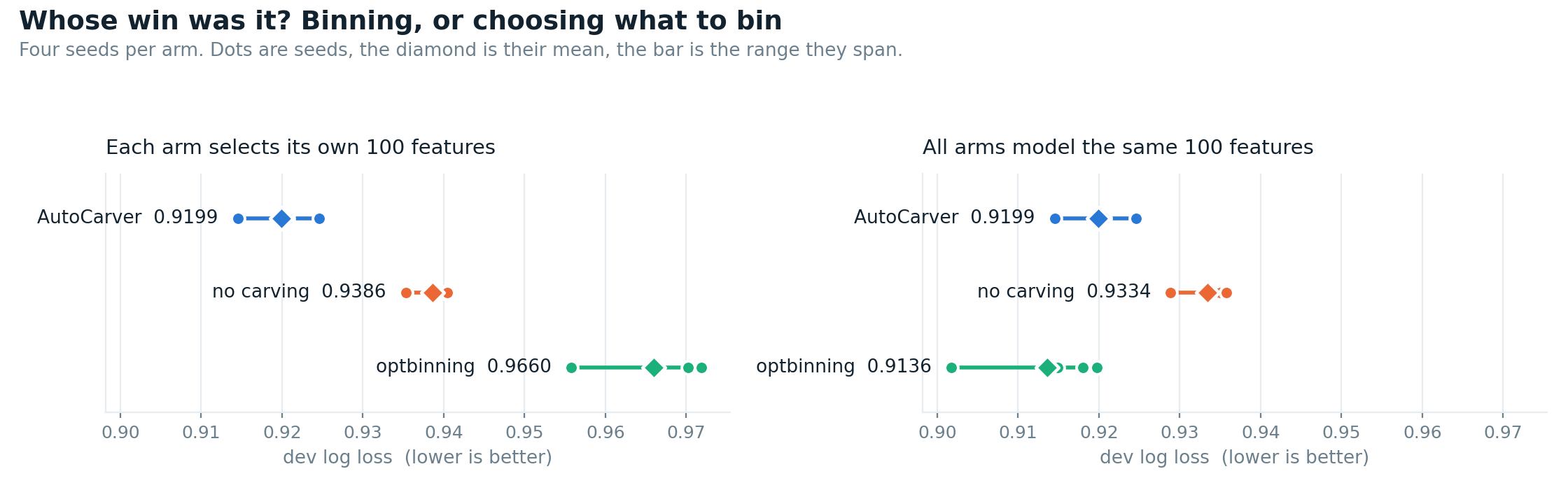
Within the left panel, every arm carves, selects its personal 100 options, then tunes. Each pair separates with no overlap: AutoCarver beats no carving by 2.45× the pooled seed unfold, no carving beats optbinning by 2.56×, and AutoCarver beats optbinning by 3.50×. In the correct panel, all three arms mannequin the identical 100 options, so solely the binning differs. AutoCarver scores the identical in each panels, for the reason that shared checklist is its personal choice. On this shared set, we discover two issues.

First, binning earned its place. Each binners beat the unbinned arm by 1.59× the pooled unfold, with no overlap, and every wins on all 4 seeds individually. We had believed this for a yr with out testing it, and it holds.

Second, the 2 libraries are indistinguishable as binners. On an identical options, the hole between them is 0.0063 of log loss, which is 0.45× their pooled unfold, and their ranges overlap. Equalising the choice strikes the three.50× pipeline win by 0.05 of log loss and reverses its signal. What separated the libraries right here was subsequently not how they lower the options, however which options their selectors saved. This shared setting additionally favours AutoCarver. The 100 options are its personal choice, and sixteen of them are ordinal bands, whose ranges have a pure order. AutoCarver and the unbinned arm use that order, whereas optbinning treats these bands as unordered classes. Even with this benefit, AutoCarver didn’t win.

We gave optbinning two extra probabilities by itself choice, and neither modifications the image. Rank-encoding the 238 ordinal bands, in order that it could possibly use the order as its documentation prescribes, helps by 0.48× the unfold (0.9660 → 0.9571). Capping it at three bins, to match AutoCarver’s realised width, makes it worse (0.9707).

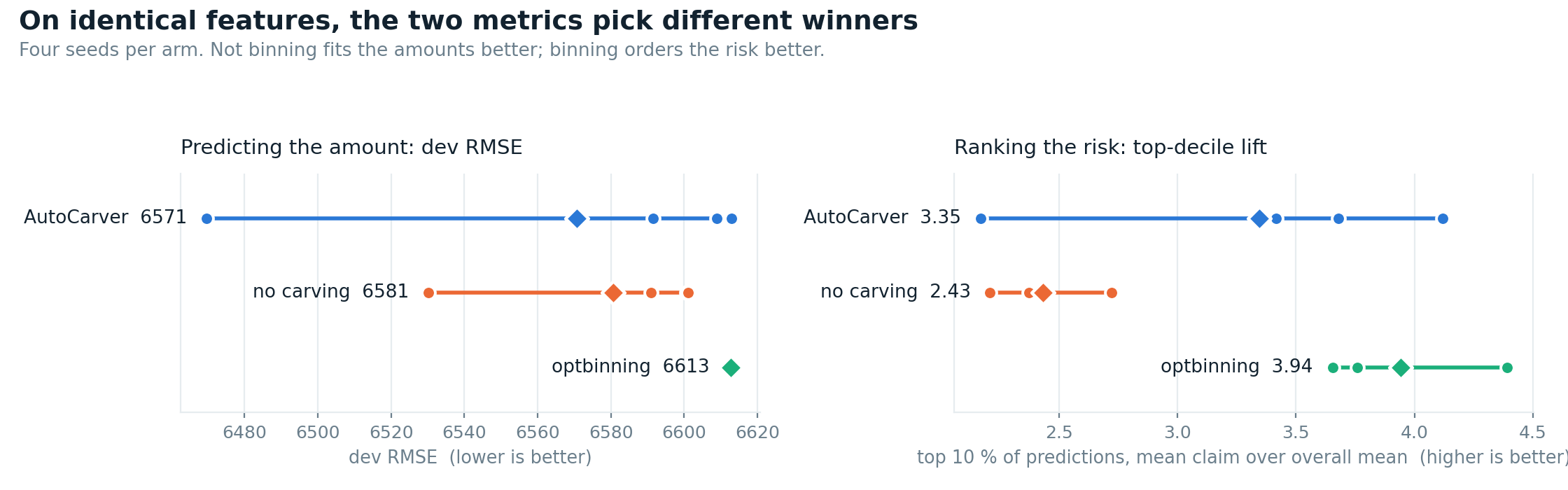
Severity wants a special metric to indicate any distinction. On the identical 200 options, dev RMSE places AutoCarver at 6570.7, no carving at 6580.7 and optbinning at 6612.8. No pair is greater than 0.89× its pooled unfold aside. A continuing predictor, the coaching imply, scores 6617.6, inside 47 of each one among them.

Prime-decile carry reveals extra. It’s the imply declare among the many 10% of insurance policies a mannequin ranks highest, divided by the general imply, so a mannequin with no sign scores 1.00. On this metric, optbinning clears the unbinned arm by 2.41× the pooled unfold. AutoCarver can be above the unbinned arm, however solely by 0.74×, which is contained in the noise. The 2 binners draw at 0.44×. The ordering is similar as for frequency, and RMSE couldn’t see it.

RMSE is blind right here as a result of it rewards overfitting on this goal. On the shared options, the binned fashions rating about the identical on prepare and dev. One unbinned mannequin, nonetheless, reached a prepare RMSE thrice decrease than its dev RMSE (1994 towards 6530). This memorising mannequin posted the perfect dev RMSE of its arm, whereas its carry stayed low, at 2.37.

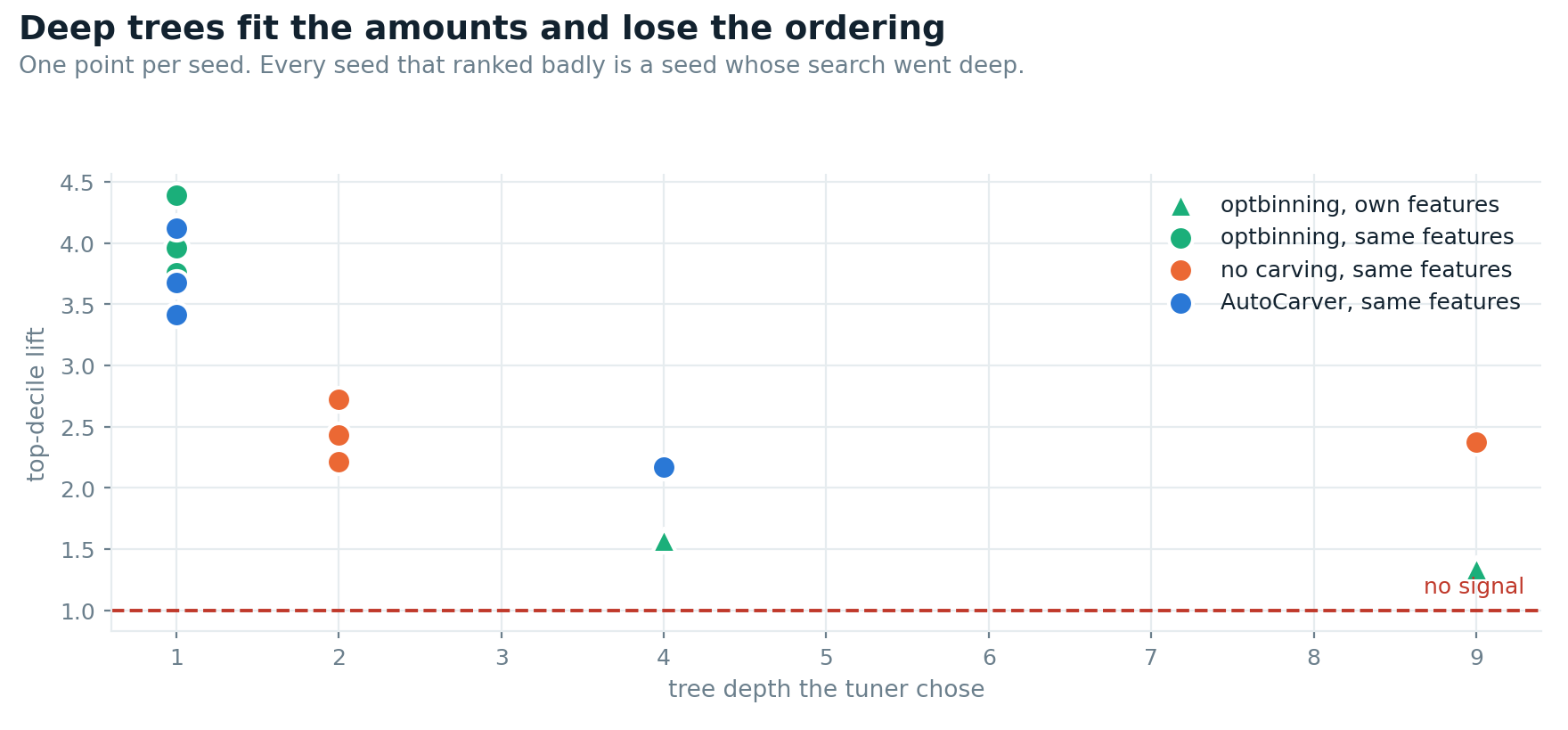
The mechanism reveals within the tree depths the tuner selected. With out binning, the search selected depth 2 on three seeds and depth 9 on the fourth. With binning, it stayed at depth 1 on seven of eight seeds. Deep bushes match the quantities and lose the ordering. Binning subsequently acted as a regulariser. On a heavy-tailed goal, this commerce fits anybody who must know which insurance policies are costly, fairly than how costly they’re. It’s a tendency, and it doesn’t all the time maintain: the one binned mannequin that went to depth 4 noticed its carry fall to 2.17.

This comparability has three limits. First, it covers one dataset and one downstream pipeline. Second, the arms solely choose the identical options when compelled to, which is why we report each comparisons. Third, each severity arm consumes the identical frequency hand-off, so the severity comparability isolates the severity binner and nothing else.

4. Takeaways

• Issue the issue. Every half will get a mannequin suited to its goal. We in contrast this with a single mannequin in the course of the competitors, on the general public leaderboard, however that comparability just isn’t reproduced right here.

• Bin the options, then examine which step paid off. Binning beat the unbinned arm by 1.59× the seed unfold, however the hole between the pipelines was seven instances the hole between the binners. Our pipeline gained on function choice.

• Verify that the metric can see the distinction. Dev RMSE couldn’t separate any severity arm from predicting the imply, and it most well-liked a mannequin that overfit threefold. Prime-decile carry separated optbinning from no carving at 2.4× the seed unfold.

• Examine with the only baseline first. For a yr, 6613.8 dev RMSE appeared like a working severity mannequin. The coaching imply scores 6617.6.

• Measure the seed unfold earlier than studying a margin. 4 additional runs per mannequin turned two obvious wins into attracts. It’s the examine we might run first subsequent time.

Every little thing behind this text

• The code, with each pocket book saved with the outputs that produced these numbers: github.com/mdefrance/caa-challenge

• The frequency and severity notebooks on Kaggle, to run with out putting in something, at a diminished tuning funds and towards a mirror of the information

• The saved 2025 fashions, to re-score the 2025 baseline

• AutoCarver: docs · supply

···

Setup: precisely what was measured

The 2025-against-2026 comparability comes from 4 pipeline runs on one machine, on 2026-08-11. The seed sweeps and the binning comparability ran in September, on the identical machine and with the identical budgets, from the scripts in instruments/.

Past the carver, the 2026 pipeline differs in its choice measures, its severity min_freq (0.02 towards 0.03) and a narrower candidate set. None of this impacts the wall-clock comparability. The 400 tuning trials had been scored on the dev set, so each dev rating is optimistic fairly than held out. Severity and CHARGE RMSE are unweighted. No leaderboard determine is quoted on this article.

The info just isn’t within the repository: the problem information come from the ENS platform or the Kaggle mirror, which additionally holds the precise BDIFF extract. With them, each 2026 run and each comparability in part 3.4 will be re-run from the repository. On our machine, with a CUDA GPU, the seeded runs reproduce precisely. On a CPU, XGBoost runs the identical pipeline however doesn’t match the final digits. The 2025 search was unseeded, so re-running the 2025 notebooks (requirements-705.txt) doesn’t give the identical numbers. As an alternative, the saved 2025 fashions are printed as a Kaggle dataset, and instruments/replay_2025_charge.py re-scores them with out re-fitting something. It reproduces the 2025 severity determine to three×10⁻⁶ and offers the 2025 CHARGE baseline. The 2025 frequency determine comes from the saved output of the 2025 pocket book.

···

References

[1] Crédit Agricole Assurances, AssurPrime : Saurez-vous prédire la prime d’assurance ? (2025), ENS Problem Information #161

[2] M. Defrance, AutoCarver (2026), PyPI / GitHub

[3] Institut nationwide de l’info géographique et forestière, Base de Données sur les Incendies de Forêts en France (BDIFF) (2025), Ministère de l’Agriculture et de la Souveraineté Alimentaire

[4] G. Navas-Palencia, OptBinning: The Python Optimum Binning library (2025), v0.21.0, GitHub

[5] M. Couillaud, Retour sur le hackathon de la Information Science Academy (2025), LinkedIn

[6] IPCC (GIEC), Local weather Change 2022: Impacts, Adaptation and Vulnerability, ch. 13 “Europe” (2022), Sixth Evaluation Report, Working Group II

[7] Swiss Re Institute, sigma 1/2026: Pure catastrophes in 2025 — the persistent rise of wildfire and storm danger (2026), sigma analysis

···

With because of Crédit Agricole Assurances and ENS Problem Information for a wonderful public competitors, to the CY Tech college students who labored via it with us, and to Zacharie Buisson for constructing the profitable answer with me.