Skewness and Kurtosis: From Moments to Machine Studying

1. Why We Want Samples: Inhabitants vs. Pattern

Would it not be sensible if I mentioned, “I need to discover out the typical marks of Class 12 college students within the Non-Medical stream throughout India”?

I imply, who’s going to go to each faculty in India, throughout each state, each district, and each village? That’s subsequent to inconceivable. And even when we one way or the other managed to gather all that knowledge, it might require an unlimited period of time, cash, and energy, with loads of alternatives for errors and inconsistencies alongside the way in which.

So, can this drawback not be solved?

Completely!

We are able to resolve it utilizing some of the vital ideas in statistics: Inhabitants vs. Pattern.

I would like you to have a look at this picture:

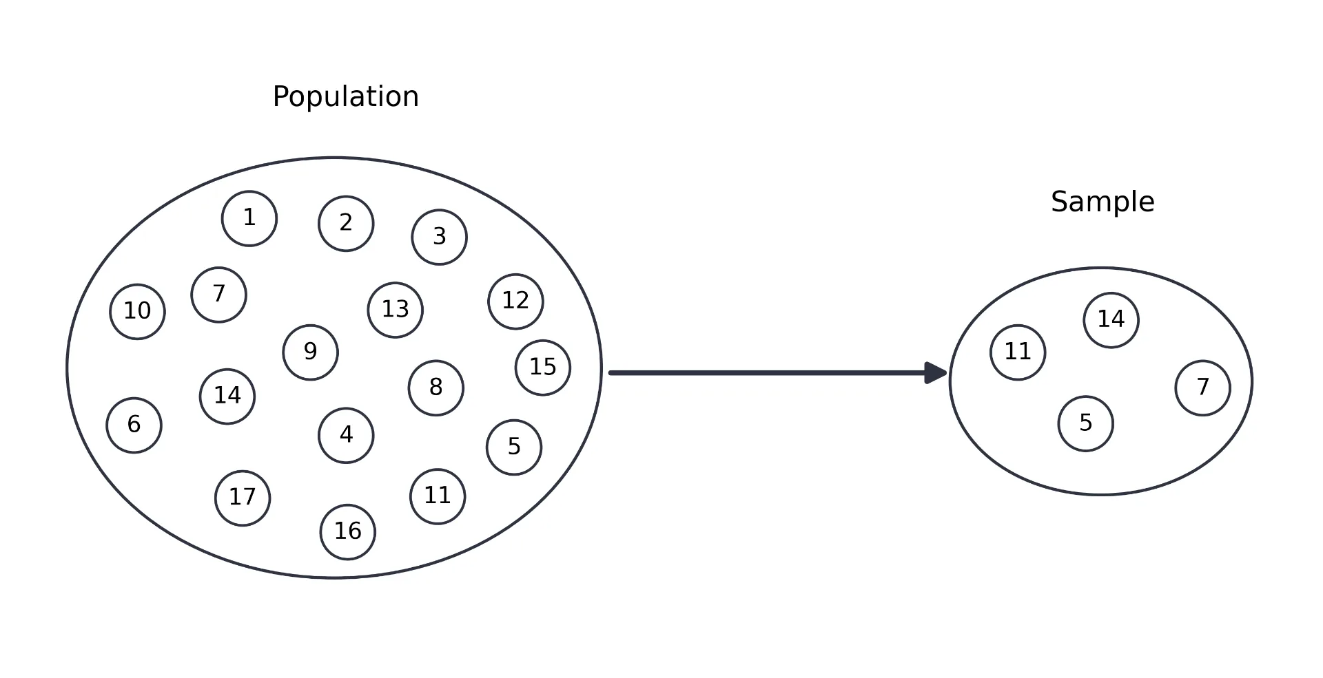
As proven above, a subset of a inhabitants is called a pattern.

When the info is just too giant to gather or compute, we regularly use pattern knowledge as an alternative. However there may be one vital situation: the pattern must be consultant of the inhabitants and shouldn’t introduce systematic bias. Because of this we must always not choose solely a selected group of individuals in a approach that would simply alter the result.

For instance, if I solely take into account college students who’ve scored 90% or above, the typical marks will naturally be very excessive. But when we take into account college students with every kind of marks, starting from low to excessive, the pattern is extra prone to signify the precise inhabitants, and subsequently, the outcomes usually tend to be nearer to the true inhabitants worth.

The dimensions of the inhabitants is denoted by N, whereas the scale of the pattern is denoted by n.

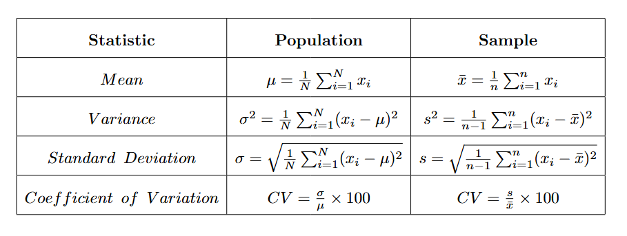
2. Why Divide by n − 1? Levels of Freedom Defined

Right here, a query might come up — why, in a pattern, are we dividing by (n-1) and never by (n)?

To clear up this confusion, we have to study one thing vital.

Do you know that the sum of deviations from the imply is at all times 0?

Here’s a small proof.

That is our pattern imply, proper?

x̄ = (x₁ + x₂ + ⋯ + xₙ) / n

If we multiply either side by (n),

n·x̄ = x₁ + x₂ + ⋯ + xₙ

After increasing, we’ll get one thing like this, which suggests the sum of the deviations of every pattern level from the imply:

(x₁ − x̄) + (x₂ − x̄) + ⋯ + (xₙ − x̄) = 0

It would at all times be 0.

Σᵢ₌₁ⁿ (xᵢ − x̄) = 0

Now, in keeping with this, let’s discover one thing.

Suppose we’ve three deviations:

-2, 0, ?

Do we actually want all three deviations?

From the opposite two, I can simply say that the third one must be (+2). That’s the one worth that can make the sum equal to 0.

So, out of those 3 deviations, we are able to independently select solely 2. The final one is routinely decided by the opposite two.

Subsequently, typically, if we’ve (n) deviations from the pattern imply, solely (n-1) of them can range independently as a result of their sum have to be 0.

And that is the place we get our first instinct for Levels of Freedom.

However there may be another vital level.

After we calculate pattern variance, we’re utilizing the pattern imply as an alternative of the true inhabitants imply. Due to this, dividing by (n) would systematically make our estimate of variance a little bit too small.

Dividing by (n-1) corrects this bias and offers us an unbiased estimate of the inhabitants variance.

And that’s how, unknowingly, you grew to become aware of the idea of Levels of Freedom.

Now you is perhaps questioning: why did we take such a protracted route by populations, samples, and levels of freedom earlier than even speaking about skewness?

As a result of skewness and kurtosis are statistical measures, and to correctly perceive their formulation, we have to perceive the place inhabitants and pattern formulation come from.

3. Moments: The Constructing Blocks of Form

Earlier than we transfer on to our primary subject, I would like us to study another vital idea first, Moments.

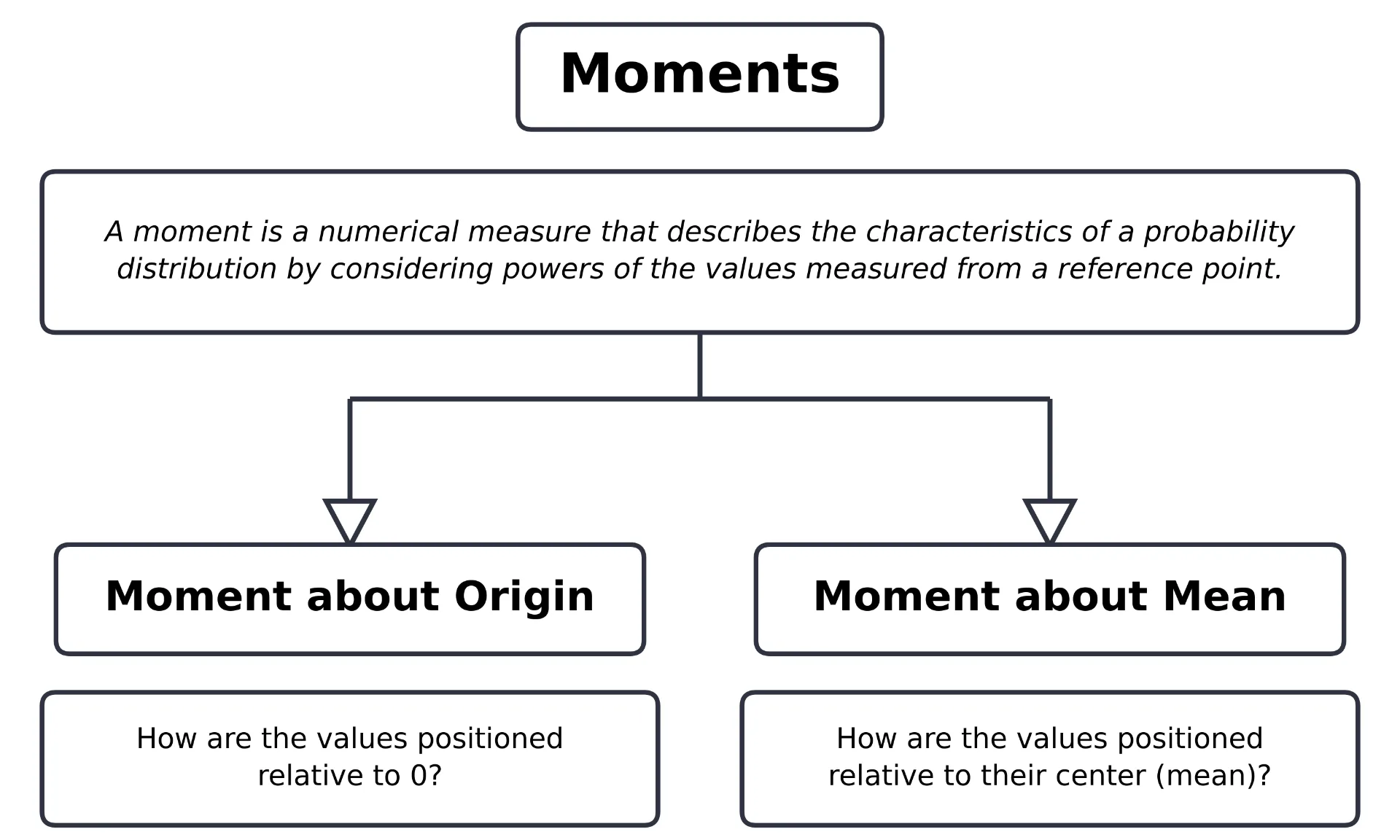
Now we have 4 central moments:

– First Central Second → 0

– Second Central Second → Variance

– Third Central Second → Associated to Skewness

– Fourth Central Second → Associated to Kurtosis

Now we have already gone by the Imply and Variance, which correspond to the first uncooked second and second central second, respectively.

For this weblog, we’ll take a deep dive into the Third and Fourth Central Moments and see how, after standardization, they result in measures of Skewness and Kurtosis.

 — First Central Second → 0 →

μ₁ = E[(X − μ)]

 — Second Central Second → Variance →

μ₂ = E[(X − μ)²]

 — Third Central Second → Associated to Skewness →

μ₃ = E[(X − μ)³]

 — Fourth Central Second → Associated to Kurtosis →

μ₄ = E[(X − μ)⁴]

These inhabitants moments are outlined utilizing the inhabitants distribution.

If we need to calculate the corresponding pattern moments, we exchange the inhabitants expectation with the corresponding pattern common.

mᵣ = (1/n) Σᵢ₌₁ⁿ (xᵢ − x̄)ʳ

4. Skewness: Measuring Asymmetry

4.1 Symmetric vs. Skewed Distributions

Now we’ve every thing we have to perceive our primary subject of curiosity, so allow us to start by first understanding what a Distribution is.

 → A distribution describes how the values of a variable are distributed and the way steadily completely different values or ranges of values happen. We are able to merely consider it as a map of our knowledge.

This map may very well be Symmetric or Non-Symmetric.

Symmetric as in:

And non-symmetric distributions are additional categorised into two sorts — right-skewed and left-skewed distributions:

Folks usually get confused as a result of they take into account the facet with extra of the distribution to be the facet akin to its identify. However there may be one key factor to recollect: at all times take a look at the tail.

If the lengthy tail extends towards the proper, then it’s Proper-Skewed (Positively Skewed).

And if the lengthy tail extends in direction of the left, then it’s Left-Skewed (Negatively Skewed).

Right here is Python code that generates 1,000 random knowledge factors, displaying right-skewed, regular, and left-skewed distributions.

import numpy as npimport matplotlib.pyplot as pltfrom scipy.stats import gaussian_kde# Generate knowledgenp.random.seed(42)# Constructive skewness (right-skewed)constructive = np.random.exponential(scale=2, dimension=1000)# Regular distributionregular = np.random.regular(loc=5, scale=1, dimension=1000)# Unfavorable skewness (left-skewed)unfavourable = -np.random.exponential(scale=2, dimension=1000)# Operate to plot distributiondef plot_distribution(knowledge, title):    # Imply    imply = np.imply(knowledge)    # Median    median = np.median(knowledge)    # KDE    kde = gaussian_kde(knowledge)    x = np.linspace(min(knowledge), max(knowledge), 1000)    y = kde(x)    # Mode = x-value the place KDE is most    mode = x[np.argmax(y)]    # Plot histogram    plt.hist(        knowledge,        bins=30,        density=True,        alpha=0.5    )    # KDE curve    plt.plot(        x,        y,        linewidth=2,        label="KDE"    )    # Imply    plt.axvline(        imply,        linewidth=2,        coloration = 'pink',        label=f"Imply = {imply:.2f}"    )    # Median    plt.axvline(        median,        linewidth=2,        coloration = 'inexperienced',        label=f"Median = {median:.2f}"    )    # Mode    plt.axvline(        mode,        linewidth=2,        coloration = 'black',        label=f"Mode ≈ {mode:.2f}"    )    plt.title(title)    plt.xlabel("Values")    plt.ylabel("Density")    plt.legend()    plt.present()# Plot all threeplot_distribution(constructive, "Constructive Skewness (Proper-Skewed)")plot_distribution(regular, "Regular Distribution")plot_distribution(unfavourable, "Unfavorable Skewness (Left-Skewed)")

4.2 Imply, Median and Mode in Skewed Information

Yet another factor we must always take a look at and observe is how the Imply, Median, and Mode are positioned in these three distributions.

For a Left-Skewed (negatively skewed) distribution -> Imply < Median < Mode.

For a symmetric regular distribution, we typically observe -> Imply ≈ Median ≈ Mode.

For Proper-Skewed (Positively skewed) distribution we regularly observe -> Imply > Median > Mode.

The stretch within the tail of a skewed distribution can typically be brought on by excessive values or outliers on one facet of the distribution. Nonetheless, skewness doesn’t at all times imply that outliers are current; the distribution itself can naturally have an extended tail on one facet.

4.3 From the Third Central Second to Skewness

So, shifting ahead, we’ve already seen a mathematical glimpse of skewness above whereas I used to be explaining the idea of Moments.

 — Third Central Second → Associated to Skewness →

μ₃ = E[(X − μ)³]

As we are able to see above, I’ve talked about it as Associated to Skewness, not Skewness itself. And that completely leads us to an vital query: Why are we standardizing it right here?

We simply must standardize it a little bit bit in order that the ensuing measure turns into unbiased of the size of the info.

γ₁ = E[(X − μ)³] / σ³

Right here, we divide the Third Central Second by the dice of the Normal Deviation.

The Third Central Second has a cubed unit, corresponding to (cm³), (km³), and many others. However we don’t need our skewness worth to rely upon the unit during which our knowledge is measured.

So, by dividing it by the dice of the Normal Deviation, we cancel out the models and get a unitless (dimensionless) worth.

Yet another vital query right here may very well be: Why do we have to use the third energy? Why not sq. it?

 (X —  μ)

represents the gap of an information level from the imply.

If we sq. this distance, each constructive and unfavourable deviations change into constructive. So, we’d lose details about the route of the deviation.

However after we dice it, one thing fascinating occurs:

(+2)³ = +8

whereas

(-2)³ = -8

The signal is preserved!

This permits the Third Central Second to seize the route of asymmetry across the imply.

There’s one other vital level right here. Cubing additionally offers a lot larger weight to giant deviations. For instance:

2³ = 8,

5³ = 125

So, excessive values have a a lot stronger affect on the Third Central Second. This is likely one of the the reason why skewness is especially delicate to excessive values and outliers.

4.4 Pattern Skewness: Fisher–Pearson and Bias Correction

Now, another vital factor to say, the formulation we noticed above is for Inhabitants knowledge.

However in most real-world issues, we not often have entry to your complete inhabitants. We often work with a Pattern.

Subsequently, we have to modify the inhabitants formulation when calculating skewness from pattern knowledge.

This adjustment leads us to the Fisher–Pearson pattern skewness coefficient.

g₁ = [(1/n) Σᵢ₌₁ⁿ (xᵢ − x̄)³] / [(1/n) Σᵢ₌₁ⁿ (xᵢ − x̄)²]^(3/2)

On wanting on the method for the primary time, it would look scary, however it’s really fairly easy.

It’s principally the third pattern central second divided by the (3/2)-power of the second pattern central second.

The instinct right here is:

– The Third Pattern Central Second tells us concerning the uneven behaviour of the info.

– The Second Pattern Central Second tells us concerning the unfold or scale of the info.

So, by dividing the third second by the (3/2) energy of the second second, we’re primarily asking,

How a lot asymmetry is there relative to the size of the info?

This standardization is vital as a result of we don’t need our skewness worth to rely upon the models or scale of the info.

However even this estimator has a limitation: it may be biased, significantly for small pattern sizes.

Give it some thought this manner, if we repeatedly take completely different samples from the identical inhabitants and calculate the skewness of every pattern, the values will fluctuate. If we take the typical of those pattern skewness estimates over many repeated samples, it could systematically differ from the precise inhabitants skewness.

We wouldn’t merely name this distinction a mistake. When an estimator systematically tends to overestimate or underestimate the amount we are attempting to estimate, this systematic distinction known as Bias.

So, we want a correction issue, let’s name it C(n).

We are able to write:

G₁ = C(n)* g₁

This correction issue is derived from the anticipated behaviour of the pattern skewness estimator underneath repeated sampling.

This leads us to the Adjusted Fisher–Pearson Skewness Coefficient.

G₁ = [√(n(n − 1)) / (n − 2)] · g₁

The adjustment barely modifications the estimate to compensate for the systematic bias current within the unadjusted pattern skewness.

And because the pattern dimension turns into very giant, the correction issue approaches (1), so:

G₁ → g₁

In different phrases, for big samples, the distinction between the adjusted and unadjusted skewness turns into very small.

Right here, as we are able to see, the correction issue solely relies on (n). However why not one thing else?

 → We don’t need to calculate a special correction primarily based on whether or not the info is measured in ₹100, ₹10,000, heights, salaries, and many others.

The issue we’re correcting is primarily a finite-sample drawback.

So, the correction ought to rely upon the Pattern Measurement moderately than the precise values or models of the info.

4.5 Tips on how to Interpret Skewness Values

Now, the very last thing we have to focus on is the worth of skewness we’ll get.

How will we classify whether or not our knowledge is very skewed or mildly skewed?

There isn’t a common mathematical rule for this as a result of the interpretation of skewness relies upon closely on the context and the info.

As a tough rule of thumb:

– If Skewness ≈ 0 → the info is roughly symmetric.

– If Skewness is constructive → the distribution is Proper-Skewed.

– If Skewness is unfavourable → the distribution is Left-Skewed.

– If |Skewness| is giant → the distribution reveals a stronger diploma of asymmetry.

However context issues.

A skewness worth of 1 is perhaps completely acceptable in a single context and problematic in one other. There isn’t a single cutoff that may inform us whether or not skewness is “good” or “dangerous” for each dataset.

Allow us to see this by Python code as effectively, utilizing the identical random dataset I confirmed above.

from scipy.stats import skewprint("Constructive skewness:", skew(constructive))print("Regular skewness:", skew(regular))print("Unfavorable skewness:", skew(unfavourable))

Constructive skewness: 1.865034222864843

Regular skewness: -0.036662811518565

Unfavorable skewness: -1.6510942321423066

From the above outcomes, we are able to clearly see that the ’+’ and ‘-’ indicators present us the route of skewness.

We are able to additionally see that the Regular Skewness is barely unfavourable. We are able to deal with it as roughly symmetric. Nonetheless, a skewness worth near zero alone doesn’t show that the distribution is usually distributed. Subsequently, we’d not take into account this distribution to be meaningfully left-skewed primarily based on its skewness worth alone.

We are able to additionally clearly see that the Constructive Skewness is larger in magnitude than the Unfavorable Skewness.

However bear in mind, we do not evaluate them just because a constructive quantity is larger than a unfavourable quantity. As an alternative, when evaluating the power or magnitude of skewness, we take a look at their absolute values.

For instance:

|1.865034222864843| > |-1.651094232142306|

So, the positive-skewed distribution has barely stronger skewness than the negative-skewed distribution.

The vital factor to recollect is:

Signal → Path of skewness

Absolute worth → Magnitude or power of skewness

5. Kurtosis: It’s About Tails, Not Peaks

5.1 What Kurtosis Actually Measures

Whereas going by many websites and researching about Kurtosis, I bought to know that individuals often describe it because the “peakedness” of a distribution.

However is it actually so?

Not precisely.

Kurtosis is a standardized fourth central second that’s significantly delicate to excessive observations and tail behaviour.

In easy phrases, it helps us perceive the relative significance of utmost observations and tail behaviour.

Within the above picture, are you able to give attention to the completely different patterns of the tails?

Sure, these variations in tail behaviour are associated to Kurtosis.

As we realized earlier on this weblog whereas understanding the formulation of Skewness, an identical sample applies to Kurtosis as effectively.

β₂ = E[(X − μ)⁴] / σ⁴

which on increasing will give us:

β₂ = E[(X − μ)⁴] / (E[(X − μ)²])²

Right here, we merely take the Fourth Central Second and, to standardize it, divide it by the fourth energy of the Normal Deviation.

Right here is a straightforward flowchart to assist us bear in mind it successfully.

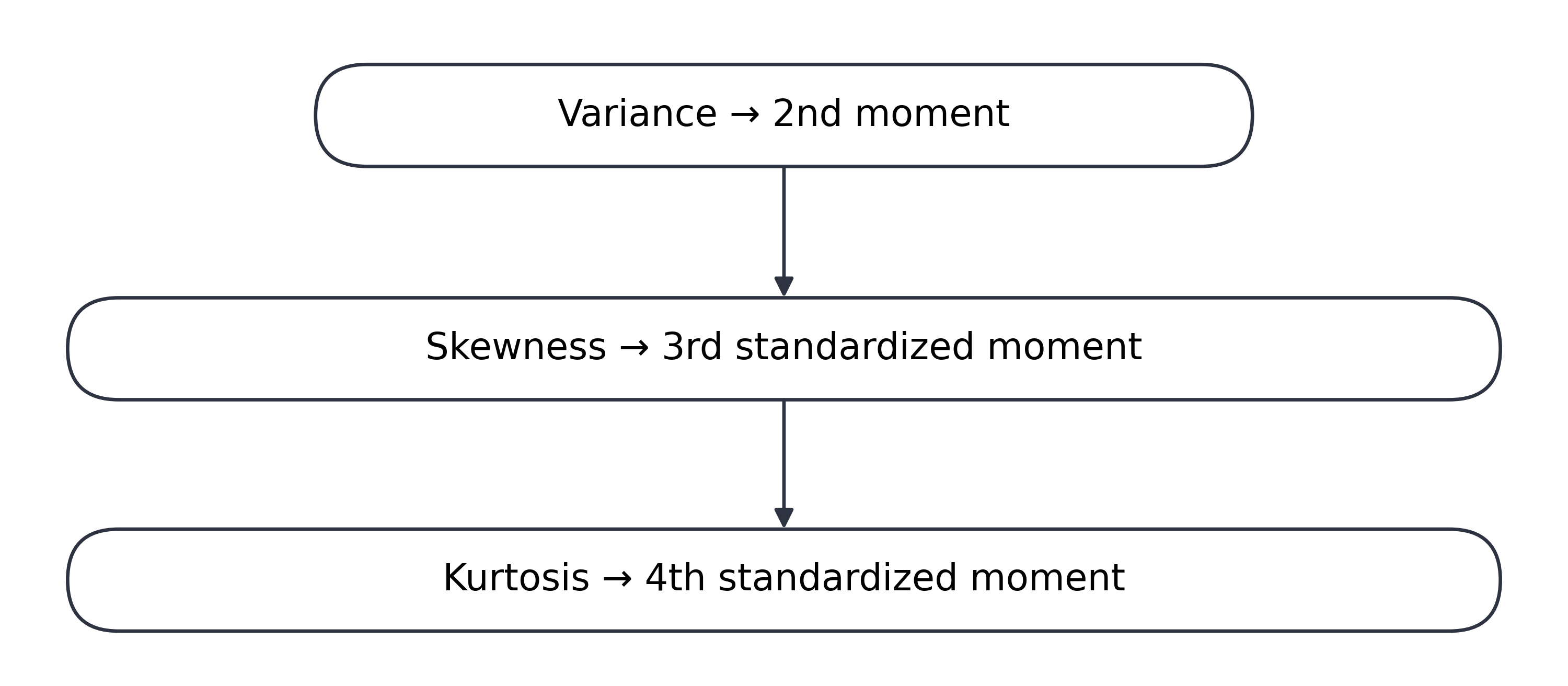
However as we all know, this formulation is for Inhabitants knowledge, and we often would not have entry to your complete inhabitants. So, we want a Pattern method to use.

However earlier than getting there, I would like us to study another vital idea, Extra Kurtosis.

5.2 Why the Fourth Energy?

Earlier than going additional, one other query might come up right here:

Why the 4th energy?

As we needed to know the route in Skewness, we used the third energy, which preserves the signal of the deviation.

However right here, we would like deviations on either side of the imply to contribute positively, whereas additionally giving a lot larger weight to giant deviations. The 4th energy does precisely that.

For instance:

(-2)⁴ = 16

and

(2)⁴ = 16

So, each constructive and unfavourable deviations contribute positively.

However that’s not the one cause we use the 4th energy.

The fourth energy additionally offers excessive values a disproportionately giant weight.

For instance:

10⁴ = 10,000

Because of this as an remark will get farther away from the imply, its contribution to the Fourth Central Second will increase very quickly.

So, Kurtosis doesn’t simply care that an remark is much away, the fourth energy makes it care way more because the remark will get farther away.

5.3 Extra Kurtosis: The place Does the “3” Come From?

Now, let’s transfer in direction of Extra Kurtosis.

To grasp Extra Kurtosis, we first want to have a look at the completely different values of Kurtosis:

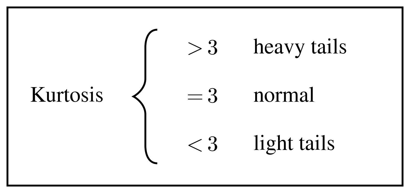
And to grasp the place this 3 got here from, we should know a little bit extra concerning the Regular Distribution.

Z = (X − μ) / σ

That is the Normal Regular Random Variable, which is obtained after we take any level (X) from a traditional distribution, subtract the imply, and divide it by the commonplace deviation:

This transformation known as standardization.

It turns into a particular case of the Regular Distribution when the imply is (0) and the usual deviation is (1) i.e.

Z ~ N(0,1)

So, for the Normal Regular Distribution, the imply is (0) and the usual deviation is (1).

Now, for Kurtosis, we have an interest within the Fourth Central Second:

E[(X − μ)⁴] = E[(σZ)⁴] = σ⁴ E[Z⁴]

For a Normal Regular Random Variable, the even moments comply with a really fascinating sample:

E[Z²ᵏ] = (2k − 1)!!

For ok = 2, we’re coping with the Fourth Second.

Right here, !! represents the Double Factorial, which suggests we multiply each different quantity as we transfer downward:

3!! = 3 × 1 = 3

And that’s the place our well-known 3 comes from!

Ok = E[(X − μ)⁴] / σ⁴ = 3σ⁴ / σ⁴ = 3

So, we are able to say that the kurtosis of a Regular Distribution is 3.

That’s why we use 3 because the baseline when decoding Kurtosis.

Nonetheless, the uncooked Kurtosis values are usually not at all times very intuitive to interpret. For instance, saying {that a} distribution has a Kurtosis of 5 doesn’t instantly inform us a lot.

So, we make the interpretation simpler by subtracting the Regular Distribution’s Kurtosis, which is 3.

Subsequently:

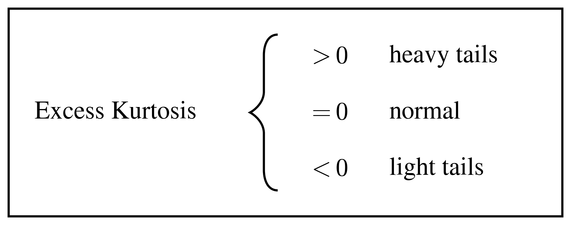
Now the interpretation turns into a lot less complicated:

– Extra Kurtosis (> 0) → typically signifies heavier tails and larger sensitivity to excessive observations than the Regular Distribution

– Extra Kurtosis (= 0) → identical kurtosis because the Regular Distribution

– Extra Kurtosis (< 0) → typically signifies lighter tails and fewer sensitivity to excessive observations than the Regular Distribution

5.4 Leptokurtic, Mesokurtic and Platykurtic Distributions

Allow us to see this by graphs:

As we are able to clearly see within the above graph, the worth of Extra Kurtosis = 20.52, which could be very excessive in comparison with 0.

This means that the distribution has larger kurtosis and sometimes heavier tails, with larger sensitivity to excessive observations than a Regular Distribution. Such a distribution is usually known as Leptokurtic.

Right here, the Extra Kurtosis = -0.01, which could be very near 0.

This tells us that the distribution has roughly the identical kurtosis as a Regular Distribution, so we are able to take into account it roughly Mesokurtic. Nonetheless, this doesn’t imply that the distribution is essentially usually distributed.

Right here, the Extra Kurtosis = -1.18.

For the reason that extra kurtosis is unfavourable, the distribution has decrease kurtosis than a Regular Distribution and sometimes much less affect from excessive observations. Such a distribution is usually known as Platykurtic.

As you possibly can see, these variations within the tails are additionally fairly evident from the graphs themselves.

Right here is the Python code used to generate the above graphs:

import numpy as npimport matplotlib.pyplot as pltfrom scipy.stats import kurtosis, gaussian_kdenp.random.seed(42)# 1. Heavy-tailed distributionheavy = np.random.standard_t(df=3, dimension=10000)# 2. Regular distributionregular = np.random.regular(loc=0, scale=1, dimension=10000)# 3. Gentle-tailed distributionmild = np.random.uniform(-2, 2, dimension=10000)# Calculate extra kurtosisprint("Heavy-tail kurtosis:", kurtosis(heavy))print("Regular kurtosis:", kurtosis(regular))print("Gentle-tail kurtosis:", kurtosis(mild))# -------------------------# Heavy-tailed distribution# -------------------------plt.determine(figsize=(8, 5))plt.hist(heavy, bins=100, density=True, alpha=0.6)# KDEx = np.linspace(-10, 10, 1000)kde = gaussian_kde(heavy)plt.plot(x, kde(x), linewidth=2)plt.title(f"Heavy-Tailed DistributionnExcess Kurtosis = {kurtosis(heavy):.2f}")plt.xlabel("Worth")plt.ylabel("Density")plt.present()# -------------------------# Regular distribution# -------------------------plt.determine(figsize=(8, 5))plt.hist(regular, bins=50, density=True, alpha=0.6)# KDEx = np.linspace(-4, 4, 1000)kde = gaussian_kde(regular)plt.plot(x, kde(x), linewidth=2)plt.title(f"Regular DistributionnExcess Kurtosis = {kurtosis(regular):.2f}")plt.xlabel("Worth")plt.ylabel("Density")plt.present()# -------------------------# Gentle-tailed distribution# -------------------------plt.determine(figsize=(8, 5))plt.hist(mild, bins=50, density=True, alpha=0.6)# KDEx = np.linspace(-2.5, 2.5, 1000)kde = gaussian_kde(mild)plt.plot(x, kde(x), linewidth=2)plt.title(f"Gentle-Tailed DistributionnExcess Kurtosis = {kurtosis(mild):.2f}")plt.xlabel("Worth")plt.ylabel("Density")plt.present()

By default, SciPy’s kurtosis() perform returns Fisher’s extra kurtosis, the place the Regular Distribution has a price of 0.

5.5 Pattern Kurtosis and Fisher’s Correction

Now, as we’re clear about Extra Kurtosis, we are literally one step nearer to our Pattern Information method for Kurtosis.

g₂ = m₄ / m₂² − 3

m₂ = (1/n) Σᵢ₌₁ⁿ (xᵢ − x̄)²

m₄ = (1/n) Σᵢ₌₁ⁿ (xᵢ − x̄)⁴

Right here, (g₂) represents the pattern extra kurtosis.

As we realized earlier, we get hold of extra kurtosis by dividing the Fourth Central Second by the sq. of the Second Central Second after which subtracting 3, the kurtosis of a Regular Distribution.

However similar to we noticed with Skewness, this estimator has a small-sample bias.

Subsequently, we apply a correction to acquire the Bias-Corrected Pattern Extra Kurtosis, often known as Fisher’s correction.

G₂ = [(n − 1) / ((n − 2)(n − 3))] · [(n + 1)(m₄/m₂² − 3) + 6]

That is the Bias-Corrected Pattern Extra Kurtosis (Fisher’s correction).

 One final vital factor to remember earlier than we transfer on.

As I discussed earlier than, individuals usually affiliate Kurtosis with peakedness. However this isn’t at all times true and shouldn’t be the centre of its definition.

Two distributions can have comparable peaks however very completely different tail behaviour.

Subsequently:

Kurtosis is strongly associated to tail behaviour and the affect of utmost observations, moderately than merely being a measure of peak top.

5.6 Skewness vs. Kurtosis: The Reminiscence Map

And with that, I’ll finish this part with a Reminiscence Map for you all.

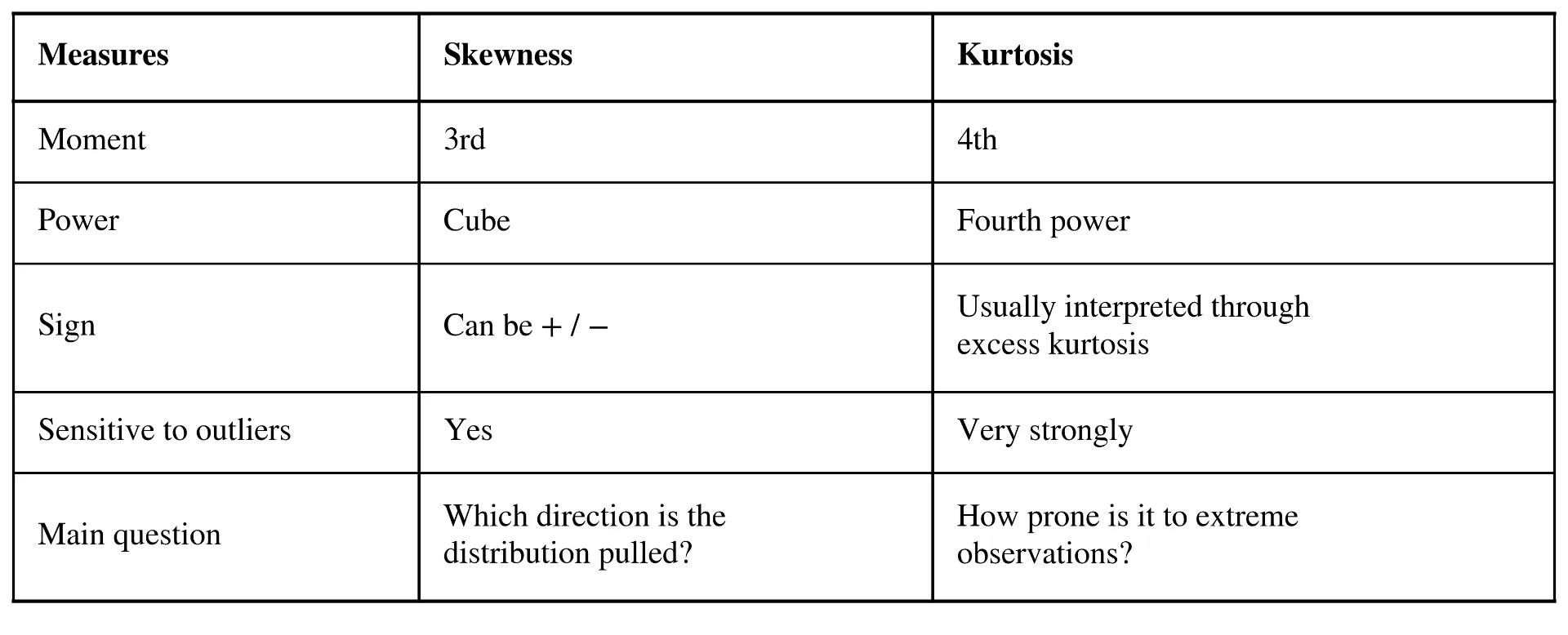
A delicate however VERY vital level

A distribution can have Excessive Skewness however Low Kurtosis, or Low Skewness however Excessive Kurtosis.

Why?

As a result of Skewness and Kurtosis measure two completely different points of a distribution:

– Skewness → tells us concerning the asymmetry and route of the distribution.

– Kurtosis → tells us concerning the behaviour of utmost values and the tails.

So, a distribution might be nearly completely symmetric whereas nonetheless having very heavy or very mild tails.

A key factor to recollect is that symmetry doesn’t inform us something concerning the behaviour of utmost values.

6. Calculating Skewness and Kurtosis in Python

I’ve supplied the Python codes above, however as soon as once more, I’ll provide the capabilities we are able to use to calculate Skewness and Kurtosis.

import pandas as pddf["variable"].skew()df["variable"].kurt()

The pandas kurt() perform returns Fisher’s pattern extra kurtosis with a bias correction by default.

from scipy.stats import skew, kurtosisskew(df["variable"])kurtosis(df["variable"])

By default, SciPy’s skew() calculates the biased pattern skewness, whereas kurtosis() returns the biased Fisher extra kurtosis except the corresponding bias correction choices are modified.

7. Taming Skewness: Information Transformations

Can we decide whether or not our knowledge is good or dangerous simply by wanting on the worth of Skewness?

Earlier than coming to any conclusion, we should first ask,

Is the skewness real? Is it brought on by excessive values or outliers? Does it really have an effect on our evaluation or the ML algorithm we’re going to use? Or might a metamorphosis assist?

Skewness itself isn’t essentially an issue. Its significance relies on the character of the info, the aim of the evaluation, and the ML algorithm getting used.

As I discussed above, we are able to apply completely different Transformations to cut back skewness. Now, let’s focus on them one after the other.

7.1 Log Transformation

Because the identify itself suggests, we take the logarithm of the values.

A log transformation compresses giant values extra strongly than smaller values, which may considerably cut back robust proper skewness.

Why not often for Left Skewness?

The usual logarithm is outlined just for constructive values, so we can’t instantly apply it to knowledge containing zero or unfavourable values.

For left-skewed knowledge, we might have to contemplate a special transformation, relying on the character of the info.

7.2 Sq. Root Transformation

Once more, because the identify suggests, we take the sq. root of the values.

It compresses bigger values, however much less aggressively than a logarithmic transformation, so it may be helpful for reasonable proper skewness.

Nonetheless, it requires non-negative values.

7.3 Dice Root Transformation

Right here, we take the dice root of the values.

One helpful property of the dice root is that it may be utilized to unfavourable in addition to constructive values.

Subsequently, it may be helpful for lowering each proper and left skewness, relying on the info.

7.4 Field-Cox Transformation

The Field-Cox Transformation is called after the 2 statisticians who launched the strategy, George Field and David Cox.

It’s a statistical approach that searches for an acceptable worth of ( λ ) to remodel the info, usually with the purpose of constructing the distribution extra symmetric or bettering the assumptions of a statistical mannequin.

The transformation is:

X^(λ) = (X^λ − 1)/λ, if λ ≠ 0
X^(λ) = ln(X), if λ = 0

If:

λ = 0

Field–Cox transformation corresponds to a logarithmic transformation.

For:

λ ≠ 0

the corresponding energy transformation is utilized.

One vital limitation to recollect is that the usual Field-Cox transformation requires strictly constructive knowledge.

Here’s a Python instance displaying how these transformations work:

import numpy as npimport matplotlib.pyplot as pltfrom scipy.stats import boxcoximport seaborn as sns# Skewed constructive knowledgeX = np.array([    10, 12, 15, 18, 20, 25,    30, 40, 60, 100, 150, 300])# Apply Field-Cox transformationX_boxcox, lambda_boxcox = boxcox(X)print("Field-Cox lambda:", lambda_boxcox)# Create plotsplt.determine(figsize=(12, 5))# Authentic knowledgeplt.subplot(1, 2, 1)sns.histplot(X, kde=True, bins=8, stat="density")plt.title("Authentic Information")plt.xlabel("Worth")plt.ylabel("Density")# Field-Cox remodeled knowledgeplt.subplot(1, 2, 2)sns.histplot(X_boxcox, kde=True, bins=8, stat="density")plt.title(f"Field-Cox Remodeled (λ = {lambda_boxcox:.2f})")plt.xlabel("Remodeled Worth")plt.ylabel("Density")plt.tight_layout()plt.present()

Field-Cox λ : -0.3978727501273978

7.5 Yeo-Johnson Transformation

The Yeo-Johnson Transformation is called after the researchers In-Kwon Yeo and Richard A. Johnson, who launched the strategy in 2000.

The Yeo–Johnson transformation is comparable in objective to the Field–Cox transformation, however it may possibly deal with zero and unfavourable values i.e.

X > 0 , X = 0 , X < 0

So, not like Field-Cox, the Yeo-Johnson Transformation might be utilized to knowledge containing constructive, zero, and unfavourable values.

The purpose stays comparable, to discover a appropriate transformation that may cut back skewness and make the distribution extra symmetric.

Right here is the Python code instance for you:

import numpy as npimport matplotlib.pyplot as pltfrom scipy.stats import yeojohnsonimport seaborn as sns# Information containing unfavourable, zero and constructive valuesX = np.array([    -100, -50, -30, -20, -10,    -5, 0, 2, 5, 10, 20, 50, 100, 200])# Apply Yeo-JohnsonX_yeojohnson, lambda_yeojohnson = yeojohnson(X)print("Yeo-Johnson lambda:", lambda_yeojohnson)# Create plotsplt.determine(figsize=(12, 5))# Authentic knowledgeplt.subplot(1, 2, 1)sns.histplot(X, kde=True, bins=8)plt.title("Authentic Information")plt.xlabel("Worth")plt.ylabel("Density")# Yeo-Johnson remodeled knowledgeplt.subplot(1, 2, 2)sns.histplot(X_yeojohnson, kde=True, bins=8)plt.title(f"Yeo-Johnson Remodeled (λ = {lambda_yeojohnson:.2f})")plt.xlabel("Remodeled Worth")plt.ylabel("Density")plt.tight_layout()plt.present()

Yeo-Johnson λ : 0.9090980955368206

8. Standardization vs. Transformation

One will need to have full readability about two issues right here:

Standardization vs Skewness and Standardization vs Transformation

Standardization

Z = (X − μ) / σ

Standardization transforms the info in order that its imply turns into 0 and its commonplace deviation turns into 1.

Why?

As a result of standardization modifications the situation and scale of the info however doesn’t change the distribution’s form within the sense related to measures corresponding to skewness and kurtosis.

However,

Transformation can change the form of the distribution and probably cut back skewness.

So, bear in mind:

Standardization modifications the size. Transformation can change the form.

9. Kurtosis in Machine Studying

Now that we perceive the arithmetic behind Kurtosis, an vital query stays: How can or not it’s helpful in Machine Studying?

Kurtosis may also help us examine the affect of excessive observations and tail behaviour relative to a traditional distribution.

If we observe excessive kurtosis, it offers us a cause to analyze additional.

We are able to search for:

– Outliers

– Information high quality points

– Real excessive observations

However bear in mind:

Excessive Kurtosis doesn’t routinely imply that we must always take away the intense values.

An excessive remark may very well be a real and vital a part of the info. Eradicating it with out understanding its origin can really injury our evaluation.

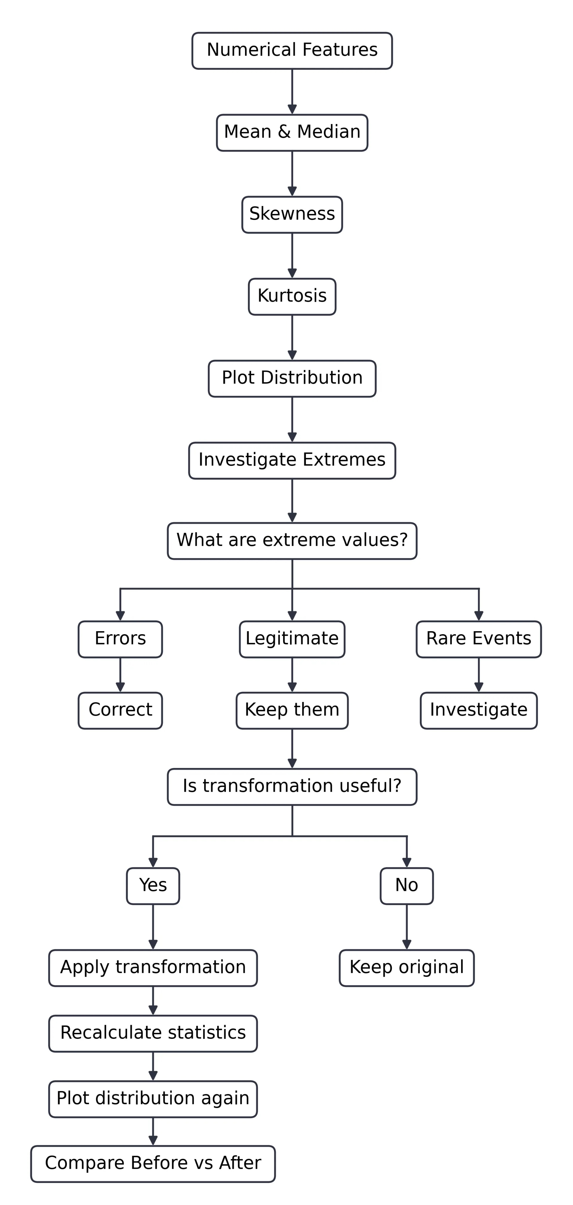
10. A Sensible EDA Workflow

For a numerical function, we are able to study ->

– Imply

– Median

– Normal Deviation

– Skewness

– Kurtosis

Then, by visualizations corresponding to ->

– Histogram

– Boxplot

– KDE Plot

– Q-Q Plot

we are able to higher perceive the distribution of our knowledge.

Collectively, these statistical summaries and visualizations kind an vital a part of Exploratory Information Evaluation (EDA).

And with that, I’ll finish this weblog with a Flowchart for EDA.

11. Supporting Supplies

The visualizations and supporting sources used on this article can be found on GitHub.

GitHub Repository

12. Assets

1. SciPy Documentation — Statistical Capabilities
   Used for the implementation and behavior of capabilities corresponding to skew(), kurtosis(), boxcox(), and yeojohnson().

2. SciPy Documentation — scipy.stats.skew
   Reference for calculating pattern skewness and understanding the bias parameter.

3. SciPy Documentation — scipy.stats.kurtosis
   Reference for Fisher’s extra kurtosis and the bias-correction choices.

4. SciPy Documentation — scipy.stats.boxcox
   Reference for the Field–Cox transformation and its implementation.

5. SciPy Documentation — scipy.stats.yeojohnson
   Reference for the Yeo–Johnson transformation and its implementation.

6. Pandas Documentation — Descriptive Statistics
   Reference for .skew() and .kurt() used within the sensible examples.

7. NIST/SEMATECH e-Handbook of Statistical Strategies
   Reference for statistical ideas together with moments, skewness, kurtosis, distributions, and exploratory knowledge evaluation.

8. George E. P. Field & David R. Cox (1964)
   An Evaluation of Transformations.
   Journal of the Royal Statistical Society: Sequence B, 26(2), 211–252.
    — Authentic paper introducing the Field–Cox transformation.

9. In-Kwon Yeo & Richard A. Johnson (2000)
   A New Household of Energy Transformations to Enhance Normality or Symmetry.
   Biometrika, 87(4), 954–959.
    — Authentic paper introducing the Yeo–Johnson transformation.

10. Joanes, D. N. & Gill, C. A. (1998)
    Evaluating Measures of Pattern Skewness and Kurtosis.
    Journal of the Royal Statistical Society: Sequence D (The Statistician), 47(1), 183–189.