Raman spectra not often go immediately from the spectrometer to a mannequin. Earlier than extracting quantitative data, we normally have to undergo some preprocessing steps, together with cropping the helpful spectral area, eradicating spikes, subtracting the baseline and normalizing the information.
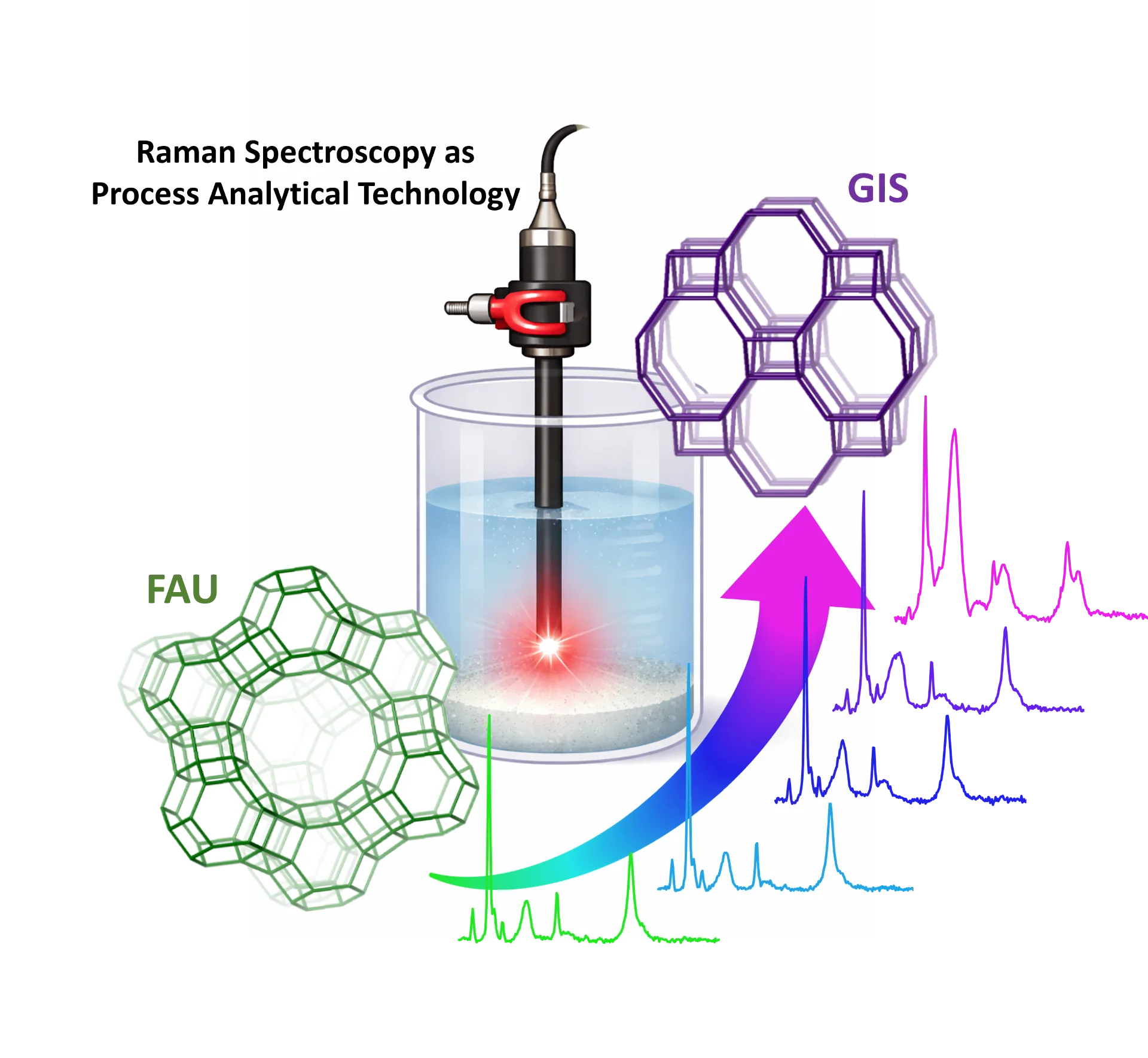
Interzeolite transformation happens throughout zeolite synthesis when one crystalline part transforms into one other, making it helpful to trace how the contribution of every part evolves with time. This course of might be tracked with Raman spectroscopy, nonetheless, the spectra have to be deconvolved. That is the place Non-Unfavorable Least Squares (NNLS) turns into significantly helpful: the measured Raman spectrum might be described as a non-negative mixture of reference spectra from the person phases.
Right here I’ll focus solely on the Raman information processing and on NNLS, ranging from the uncooked spectra and recovering the relative evolution of faujasite (FAU) and gismondine (GIS) throughout crystallization.
The entire experimental dataset is brazenly accessible in NeXus/HDF5 format on Zenodo. Additionally, this tutorial might be discovered as a Jupyter pocket book within the GitHub account of the creator.
1. Load the Raman spectra from the NeXus file
NeXus is especially handy for storing information from this experiment as a result of spectra and experimental metadata, together with crystallization time, stay saved collectively. We’ll use the file raman_crystallization_solid.nxs. Obtain it from the Zenodo document (https://doi.org/10.5281/zenodo.18972297) and place it in the identical folder as this pocket book.
So first we load the libraries for use and the information:
# If wanted:# !pip set up nexusformat scipy pybaselines matplotlibimport numpy as npimport matplotlib.pyplot as pltfrom nexusformat.nexus import nxloadfilename = "raman_crystallization_solid.nxs"root = nxload(filename)entry = root["entry"]
Let’s loop by the NeXus information teams and retailer every Raman spectrum along with its acquisition time and spectral axis:
spectra = []# Loop by the NeXus information teams and retailer every Raman spectrum along with its acquisition time and spectral axis:for identify in entry.keys(): if identify.startswith("data_"): d = entry[name] spectra.append({ "identify": identify, "time": float(np.asarray(d["time_hours"])) if "time_hours" in d else np.nan, "x": np.asarray(d["wavenumber"], dtype=float), "y": np.asarray(d["intensity"], dtype=float), })# Kind the spectra by crystallization time:spectra_all = sorted(spectra, key=lambda s: s["time"])# Retailer the crystallization instances in a NumPy array:times_all = np.array([s["time"] for s in spectra])print(f"Variety of spectra: {len(spectra_all)}")print("Instances (h):", times_all)
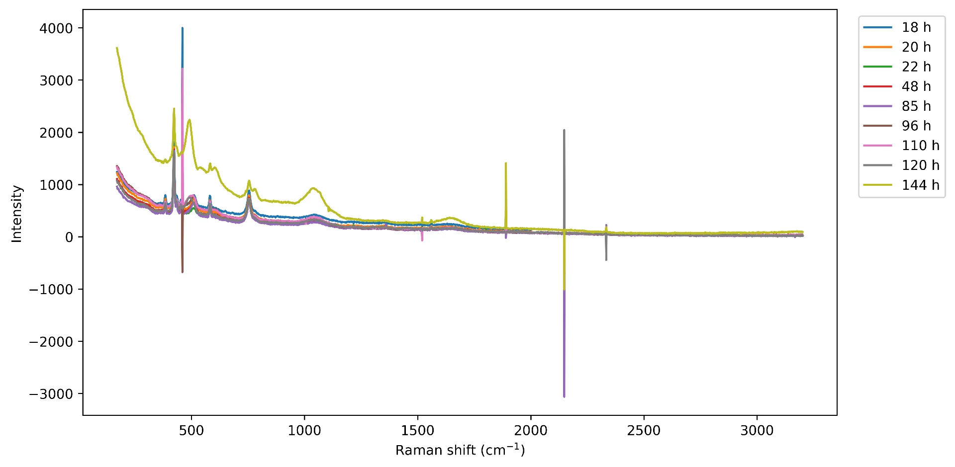
Let’s plot all of the uncooked spectra to get an concept of what we’ve:
plt.determine(figsize=(10, 5))for s in spectra: plt.plot(s["x"], s["y"], label=f"{s['time']:g} h")plt.xlabel(r"Raman shift (cm$^{-1}$)")plt.ylabel("Depth")plt.legend(bbox_to_anchor=(1.02, 1), loc="higher left")plt.tight_layout()plt.savefig("determine.png", dpi=600, bbox_inches="tight")plt.present()
The spectra acquired at 0 and 16 h weren’t used within the following evaluation, because the Raman options related to the crystalline zeolite phases weren’t but sufficiently informative. We subsequently proceed the evaluation from 18 h onward:
spectra = [s for s in spectra_all if s["time"] >= 18]instances = np.array([s["time"] for s in spectra])
2. Crop and interpolate the spectra onto a typical Raman-shift axis
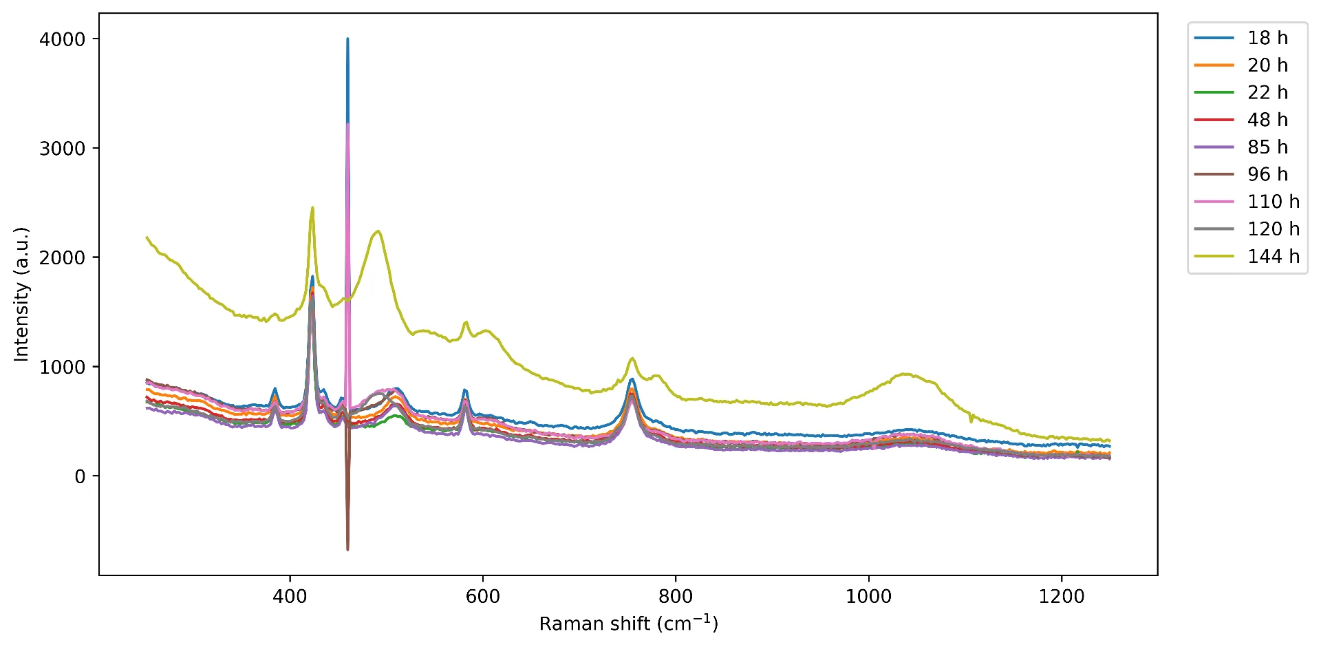
The primary preprocessing step is to take away spectral areas that we’re not going to make use of. For this dataset I preserve the 250–1250 cm⁻¹ area.
The spectra weren’t all recorded on precisely the identical Raman-shift axis, so after cropping, every spectrum is interpolated onto a typical axis. That is needed earlier than combining the spectra right into a single information matrix for the next preprocessing steps and NNLS evaluation.
Importantly, each cropping and interpolation are finished earlier than spike removing and baseline subtraction, so these algorithms solely function on the related and harmonized a part of the sign.
# ----------------------------------------------------------# Crop + interpolate all spectra to a typical Raman-shift axis# ----------------------------------------------------------low_end = 250high_end = 1250# Discover the spectral vary that's really accessible in ALL spectrax_min = max(low_end, max(np.min(s["x"]) for s in spectra))x_max = min(high_end, min(np.max(s["x"]) for s in spectra))# Use the primary spectrum because the reference axisx0 = spectra[0]["x"]mask_ref = (x0 >= x_min) & (x0 <= x_max)x_crop = x0[mask_ref]# Be certain the frequent axis goes from low to excessive Raman shiftx_crop = np.type(x_crop)Y_raw = []for s in spectra: x = s["x"] y = s["y"] # Crop every spectrum individually masks = (x >= x_min) & (x <= x_max) x_i = x[mask] y_i = y[mask] # np.interp requires growing x order = np.argsort(x_i) x_i = x_i[order] y_i = y_i[order] # Interpolate onto the frequent axis y_interp = np.interp(x_crop, x_i, y_i) Y_raw.append(y_interp)Y_raw = np.array(Y_raw)# Plotplt.determine(figsize=(10, 5))for t, y in zip(instances, Y_raw): plt.plot(x_crop, y, label=f"{t:g} h")plt.xlabel(r"Raman shift (cm$^{-1}$)")plt.ylabel("Depth (a.u.)")plt.legend(bbox_to_anchor=(1.02, 1), loc="higher left")plt.tight_layout()plt.savefig("figure_2.png", dpi=600, bbox_inches="tight")plt.present()print("Widespread Raman vary:", x_crop.min(), "-", x_crop.max(), "cm-1")print("Widespread variety of factors:", len(x_crop))print("Y_raw form:", Y_raw.form)
3. Take away spikes
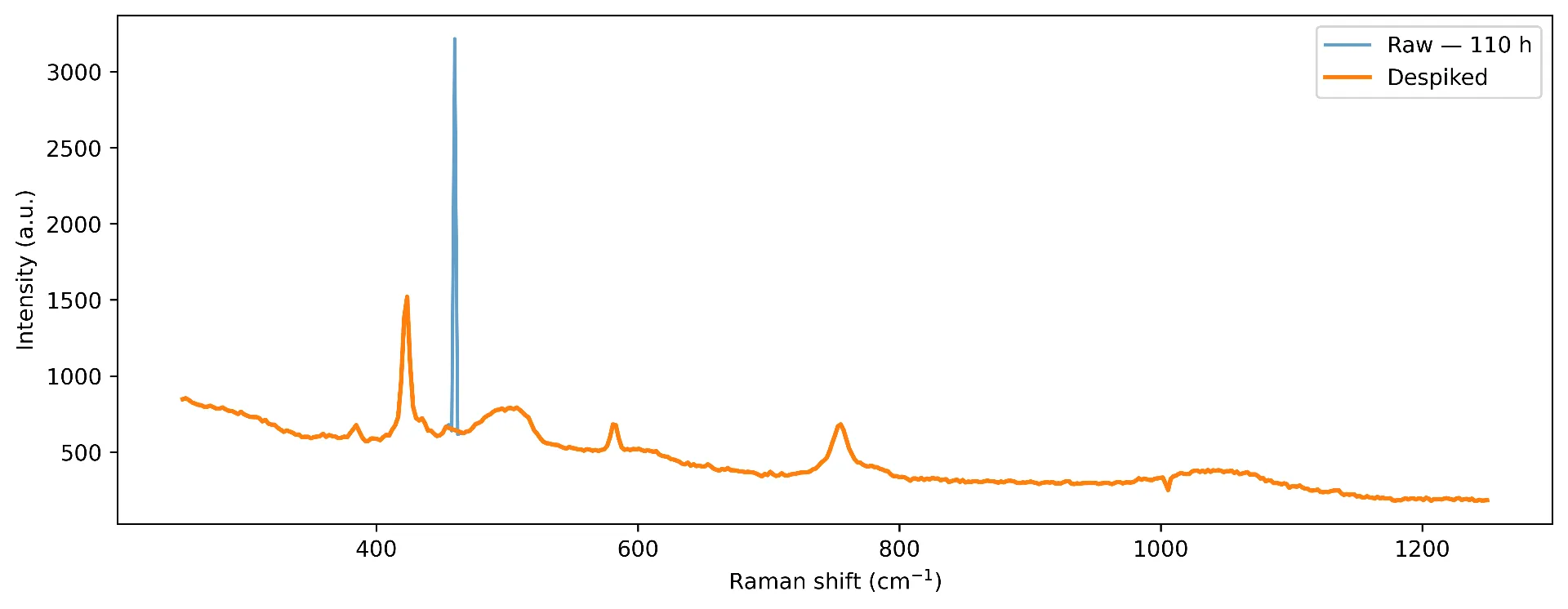
Cosmic rays and detector artifacts can generate very slender optimistic, and typically adverse, options, named spikes. A single spike can strongly have an effect on normalization or multivariate mannequin efficiency.
Right here I exploit the prominence-width spike removing method developed in “An intuitive method for spike removing in Raman spectra based mostly on peaks’ prominence and width.” The concept is intuitive: Spikes are a lot narrower than actual Raman bands. This algorithm finds all peaks within the spectra and units a threshold of their prominence and width to detect spikes. The implementation beneath additionally applies the identical logic to -y, permitting adverse spikes to be detected.
from scipy.sign import find_peaks, peak_widthsfrom scipy import interpolateimport warningsdef spike_removal( y, width_threshold, prominence_threshold, interpolation_window=10, width_param_rel=0.8, interp_kind="linear", remove_positive=True, remove_negative=True,): """Take away slender spikes from a Raman spectrum utilizing peak prominence and width. pike detection relies on the prominence/FWHM method described in: Coca-Lopez, An intuitive method for spike removing in Raman spectra based mostly on peaks' prominence and width", Analytica Chimica Acta 1295 (2024) 342312. https://doi.org/10.1016/j.aca.2024.342312 Peaks with ample prominence above 'prominence_threshold' and a width beneath 'width_threshold' are categorized as spikes and changed by interpolation from neighboring non-corrupted factors. This implementation extends the unique method by optionally detecting adverse spikes by the identical process utilized to -y. It additionally makes use of conservative checks to keep away from extrapolation or interpolation when clear information usually are not accessible on either side of a detected spike.""" y = np.asarray(y, dtype=float) def detect_spikes(sign): spike_mask = np.zeros(len(sign), dtype=bool) peaks, _ = find_peaks(sign, prominence=prominence_threshold) if len(peaks) == 0: return spike_mask widths = peak_widths(sign, peaks, rel_height=0.5)[0] width_results = peak_widths(sign, peaks, rel_height=width_param_rel) for width, left, proper in zip(widths, width_results[2], width_results[3]): if width < width_threshold: begin = max(int(np.ground(left)) - 1, 0) finish = min(int(np.ceil(proper)) + 2, len(sign)) spike_mask[start:end] = True return spike_mask spikes = np.zeros(len(y), dtype=bool) if remove_positive: spikes |= detect_spikes(y) if remove_negative: spikes |= detect_spikes(-y) if not np.any(spikes): return y.copy() y_out = y.copy() padded = np.r_[False, spikes, False] adjustments = np.diff(padded.astype(int)) begins = np.the place(adjustments == 1)[0] ends = np.the place(adjustments == -1)[0] - 1 required = {"linear": 2, "quadratic": 3, "cubic": 4} if interp_kind not in required: elevate ValueError("interp_kind have to be 'linear', 'quadratic', or 'cubic'.") skipped = [] for begin, finish in zip(begins, ends): window = np.arange( max(begin - interpolation_window, 0), min(finish + interpolation_window + 1, len(y)), ) good = window[~spikes[window]] unhealthy = np.arange(begin, finish + 1) if len(good) < required[interp_kind]: skipped.append((begin, finish, "not sufficient clear factors")) proceed if not np.any(good < begin) or not np.any(good > finish): skipped.append((begin, finish, "no clear information on either side")) proceed if unhealthy[0] < good.min() or unhealthy[-1] > good.max(): skipped.append((begin, finish, "would require extrapolation")) proceed strive: f = interpolate.interp1d( good, y[good], sort=interp_kind, bounds_error=True, ) y_out[bad] = f(unhealthy) besides ValueError: skipped.append((begin, finish, "interpolation failed")) if skipped: warnings.warn( f"{len(skipped)} spike area(s) weren't corrected as a result of " f"interpolation was thought-about unsafe: {skipped[:10]}" ) return y_out
The next cell applies the spike removing algorithm to all of the spectra and plots the spectra earlier than and after spectra spike correction. The 2 parameters value checking visually are WIDTH_THRESHOLD and PROMINENCE_THRESHOLD. They need to be tuned contemplating the spectral decision and the width of actual Raman bands.
WIDTH_THRESHOLD = 2PROMINENCE_THRESHOLD = 100WINDOW = 5Y_despiked = np.array([ spike_removal( y, width_threshold=WIDTH_THRESHOLD, prominence_threshold=PROMINENCE_THRESHOLD, interpolation_window=WINDOW, ) for y in Y_raw])# Discover spectra that have been modified by spike removingaffected = np.the place( np.any(~np.isclose(Y_raw, Y_despiked), axis=1))[0]print(f"Spectra containing corrected spikes: {len(affected)}")print("Instances:", instances[affected])# Plot each affected spectrumfor i in affected: plt.determine(figsize=(10, 4)) plt.plot( x_crop, Y_raw[i], label=f"Uncooked — {instances[i]:g} h", alpha=0.7 ) plt.plot( x_crop, Y_despiked[i], label="Despiked", lw=2 ) plt.xlabel(r"Raman shift (cm$^{-1}$)") plt.ylabel("Depth (a.u.)") plt.legend() plt.tight_layout() plt.savefig("figure_3_spike.png", dpi=600, bbox_inches="tight") plt.present()
For instance:
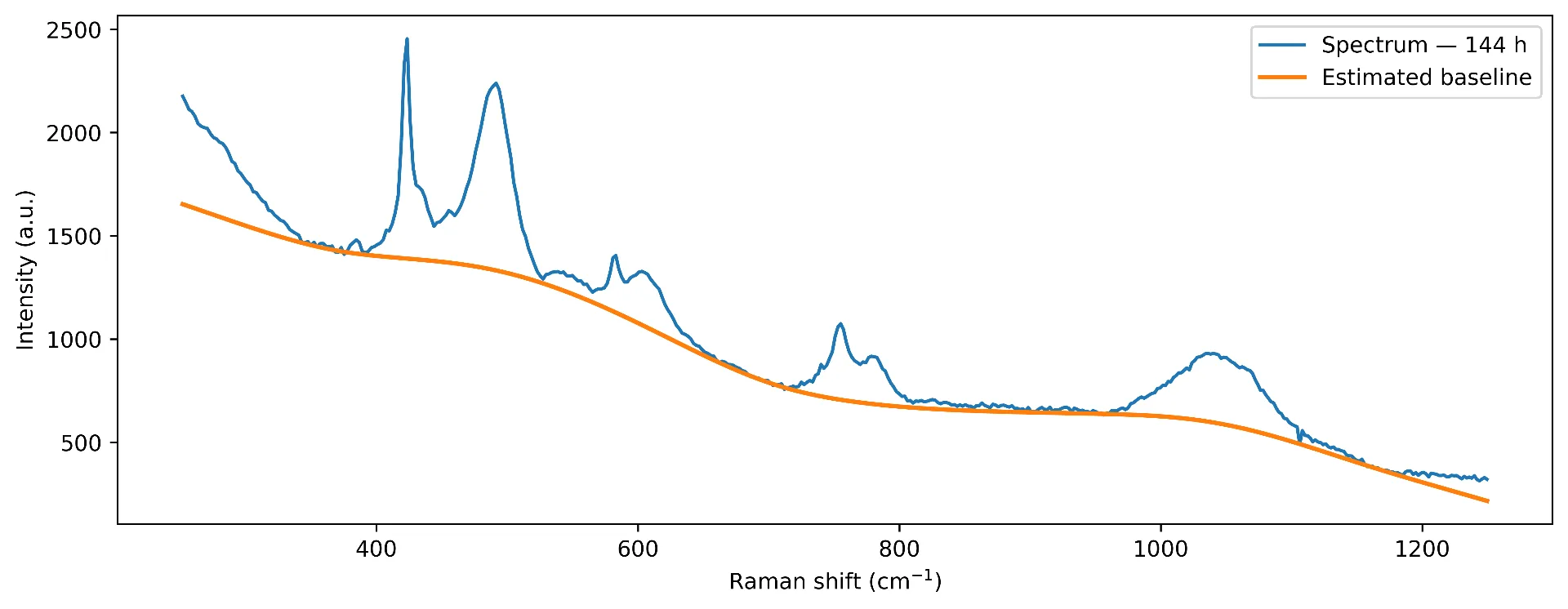
4. Baseline subtraction
The following main artifact is the slowly various spectral background. Right here I exploit uneven least squares (AsLS) baseline estimation, applied within the library pybaselines by D. Erb (https://github.com/derb12/pybaselines).
The parameters are stored near these used within the unique evaluation:
lam = 3e3: baseline smoothness.
p = 0.001: asymmetry parameter.
max_iter = 300: most iterations.
The next cell reveals the correction of the spectra:
from pybaselines import Baselinebaseline_fitter = Baseline(x_data=x_crop)baselines = []Y_corrected = []for y in Y_despiked: baseline, _ = baseline_fitter.asls( y, lam=3e3, p=0.001, max_iter=300 ) baselines.append(baseline) Y_corrected.append(y - baseline)baselines = np.array(baselines)Y_corrected = np.array(Y_corrected)# Plot all spectra with their estimated baselinesfor i in vary(len(Y_despiked)): plt.determine(figsize=(10, 4)) plt.plot(x_crop, Y_despiked[i], label=f"Spectrum — {instances[i]:g} h") plt.plot(x_crop, baselines[i], label="Estimated baseline", lw=2) plt.xlabel(r"Raman shift (cm$^{-1}$)") plt.ylabel("Depth (a.u.)") plt.legend() plt.tight_layout() plt.savefig("figure_4_baseline.png", dpi=600, bbox_inches="tight") plt.present()
For instance:
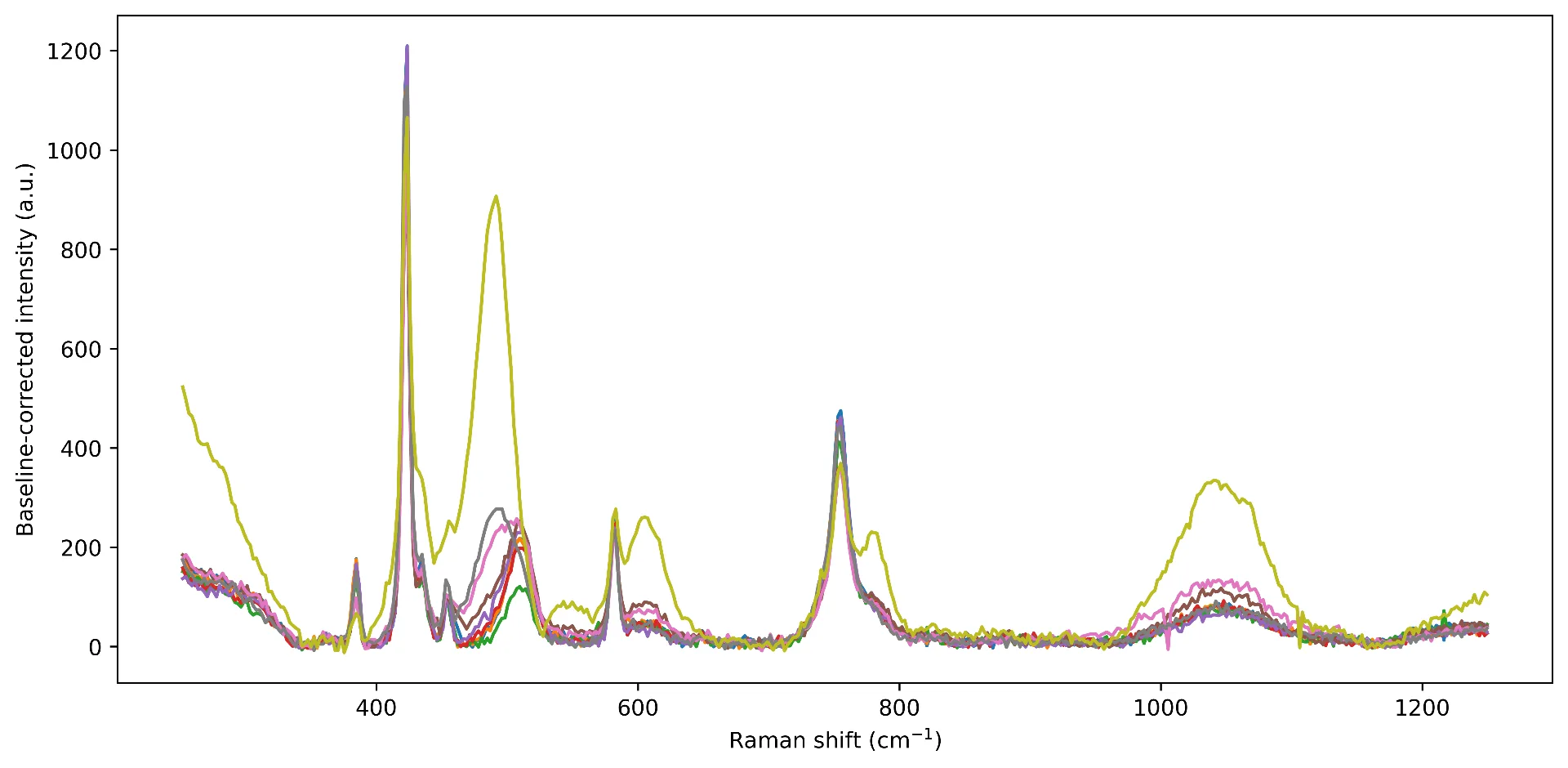
Let’s check out all spectra collectively:
plt.determine(figsize=(10, 5))for t, y in zip(instances, Y_corrected): plt.plot(x_crop, y, label=f"{t:g} h")plt.xlabel(r"Raman shift (cm$^{-1}$)")plt.ylabel("Baseline-corrected depth (a.u.)")plt.tight_layout()plt.savefig("figure_5_baselined.png", dpi=600, bbox_inches="tight")plt.present()
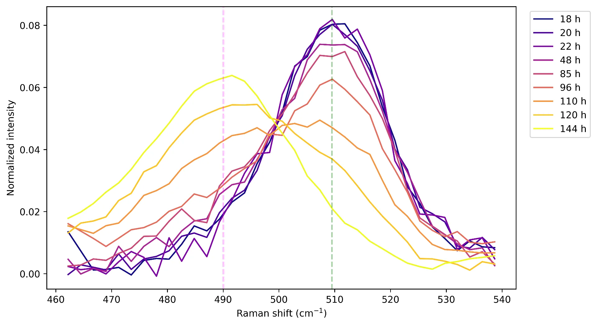
5. Give attention to the FAU/GIS diagnostic area
For the NNLS evaluation we don’t want the entire Raman spectrum. Probably the most helpful evolution happens within the slender area containing attribute FAU/GIS framework bands.
A Raman spectrum (y) containing two phases might be approximated as a linear mixture of the 2 reference spectra,SFAUand SGIS, as:
y≈CFAUSFAU+CGISSGIS
the place CFAUand CGIS are the corresponding coefficients. NNLS constrains the coefficients to be non-negative:
minc≥0∥SC−y∥22≥0
The place S is the matrix containing the spectra and C a column vector containing the coefficients. This makes NNLS engaging for easy spectral unmixing: the mannequin is quick, clear and straightforward to interpret.
Reference spectra
Right here, the spectra acquired at 18 h and 144 h are used because the FAU and GIS reference spectra, respectively. So the calculation might be finished as
from scipy.optimize import nnlsFAU_TIME = 18GIS_TIME = 144i_fau = np.argmin(np.abs(instances - FAU_TIME))i_gis = np.argmin(np.abs(instances - GIS_TIME))R = np.column_stack([Y_nnls[i_fau], Y_nnls[i_gis]])coef = np.array([nnls(R, y)[0] for y in Y_nnls])# From coefficients to weighted fractions:fractions = 100 * coef / coef.sum(axis=1, keepdims=True)fau_fraction = fractions[:, 0]gis_fraction = fractions[:, 1]
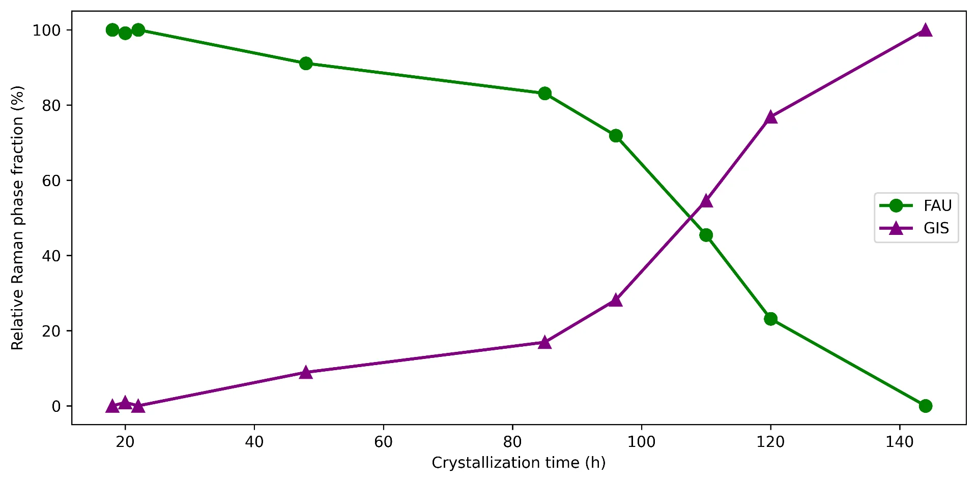
The next plot reveals the evolution of each phases:
plt.determine(figsize=(9, 4.5))plt.plot(instances, fau_fraction, "o-", shade="inexperienced", label="FAU", lw=2, ms=8)plt.plot(instances, gis_fraction, "^-", shade="purple", label="GIS", lw=2, ms=8)plt.xlabel("Crystallization time (h)")plt.ylabel("Relative Raman part fraction (%)")plt.legend()plt.present()
The NNLS outcomes clearly present the evolution of the 2 crystalline phases throughout synthesis. Initially of crystallization, the Raman sign is dominated by FAU, whereas its relative contribution progressively decreases as GIS develops. This captures the FAU → GIS interzeolite transformation and reveals how Raman spectroscopy can be utilized to observe the part evolution immediately through the synthesis.
The attention-grabbing half is that the ultimate mannequin is very simple. As soon as the spectra are correctly preprocessed, NNLS solely wants consultant spectral signatures of the person phases to get well their relative evolution through the course of.
On this instance, the mixture of Raman spectroscopy and spectral unmixing permits us to observe the transformation from FAU to GIS throughout zeolite crystallization. Within the full paper, this Raman-derived evolution is in contrast with ex situ XRD/Rietveld evaluation and varieties a part of a broader process-monitoring technique.
Extra importantly, the workflow shouldn’t be restricted to this specific synthesis. The identical normal method might be utilized as a course of analytical know-how (PAT) to different processes through which the measured spectrum evolves as a mix of recognized elements, for instance, part transformations, crystallization processes, chemical reactions or adjustments in materials composition. When appropriate reference spectra can be found, combining in situ Raman spectroscopy with data-processing strategies reminiscent of NNLS gives a comparatively easy strategy to convert advanced spectral evolution into chemically significant data.
Information and References
Primary paper N. Coca-Lopez, F. Rodriguez, L. F. Lundegaard, X. Li, E. Lozano Diz, S. B. Rasmussen, F. Tielens, M. Calatayud, M. A. Bañares, R. Portela and P. Beato, “Course of monitoring of zeolite crystallization: Bridging in situ Raman spectroscopy, ex situ XRD, and predictive machine studying fashions”, Chemical Engineering Journal 543 (2026) 177865. https://doi.org/10.1016/j.cej.2026.177865
Open dataset Course of Monitoring of Zeolite Crystallization: Bridging In situ Raman Spectroscopy, Ex situ XRD, and Predictive Machine Studying Fashions, Zenodo. https://doi.org/10.5281/zenodo.18972297
Spike removing N. Coca-Lopez, “An intuitive method for spike removing in Raman spectra based mostly on peaks’ prominence and width”, Analytica Chimica Acta 1295 (2024) 342312. https://doi.org/10.1016/j.aca.2024.342312
Evaluation on Synthetic intelligence and Raman spectroscopy N. Coca-Lopez et al., “Synthetic Intelligence-Powered Raman Spectroscopy by Open Science and FAIR Ideas”, ACS Nano 11 November 2025; 19 (44): 38189–38218. https://doi.org/10.1021/acsnano.5c09165