TL;DR
-
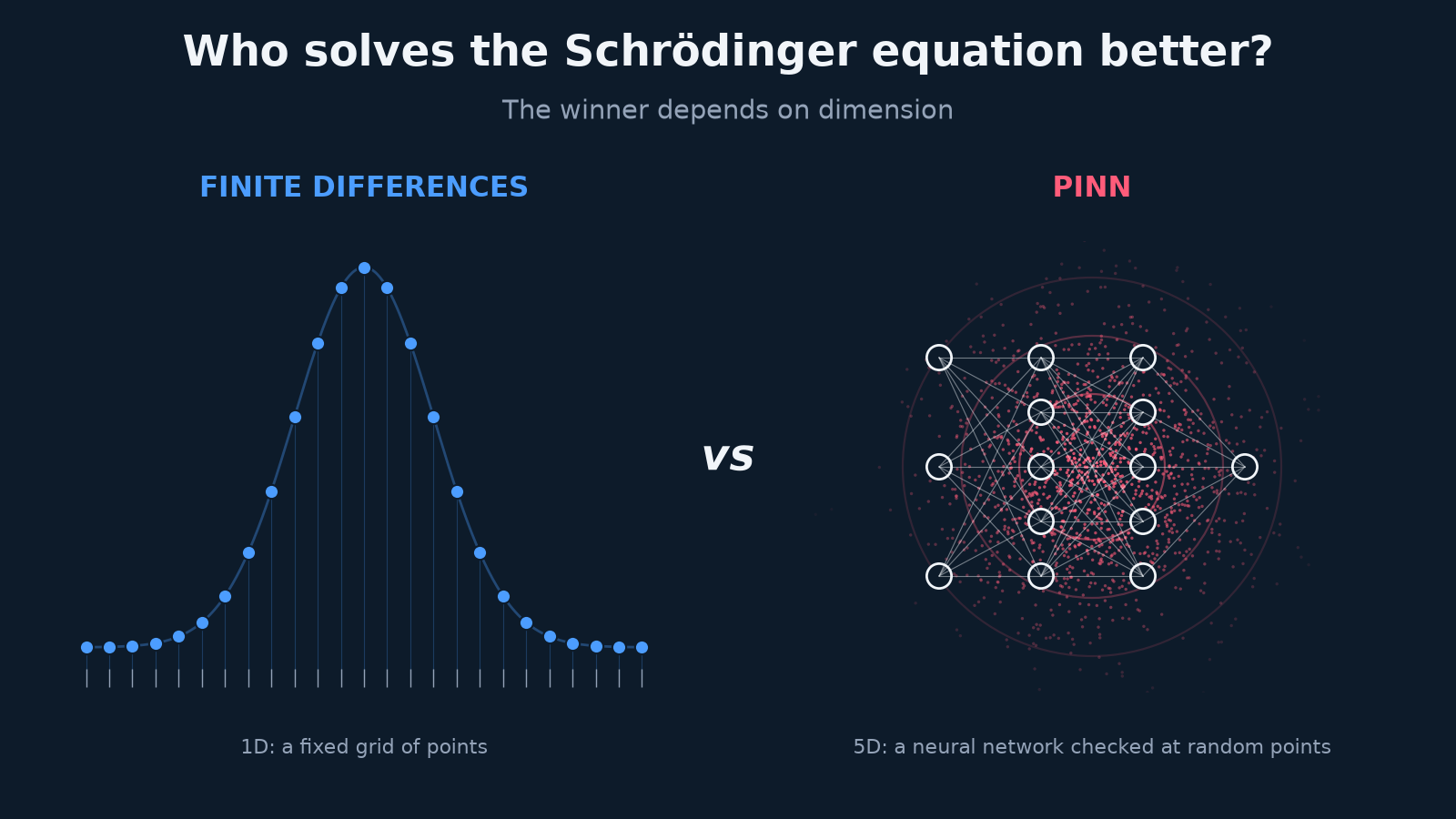
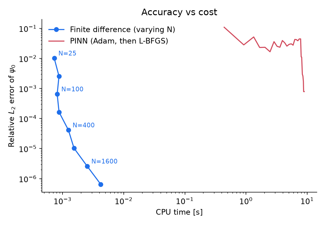
In 1D, finite variations win by about some 1000’s of occasions. They attain the PINN’s remaining accuracy in beneath a millisecond.
-
In 5D, the grid cannot compete. Matching the PINN’s 0.1% error would take about 5 billion grid factors and greater than 1 TB of reminiscence. The PINN wanted 89s of CPU time.
-
Two tips made the PINN work. Switching from Adam solely to Adam + L-BFGS reduce its error by about 50×. So, forcing ψ > 0 stopped it from converging to an excited state.
Physics-informed neural networks, or PINNs, are all over the place proper now. The idea is easy and straightforward to know. You do not want a mesh or a particular solver. You write the equation into the loss operate, and the community learns the reply.
I work in computational physics, and I saved asking one query: higher than what? Many PINN demos by no means evaluate in opposition to a great classical technique. A 2024 examine in Nature Machine Intelligence discovered that weak baselines are widespread on this discipline, and that they make machine-learning solvers look higher than they’re. So I ran the take a look at myself.
I picked an issue with a precise reply, the quantum harmonic oscillator. That means I can measure the error with none guessing. I solved it twice, first in a single dimension after which in 5. The 2 solutions turned out to be very completely different.
The issue
Image a marble rolling in a bowl. In on a regular basis physics, the marble can have any power in any respect. A quantum particle cannot. It might solely sit on sure power “rungs”, like steps on a ladder. Every rung has its personal form, known as a wavefunction ψ(x). The sq. of ψ tells you the place the particle is prone to be discovered.
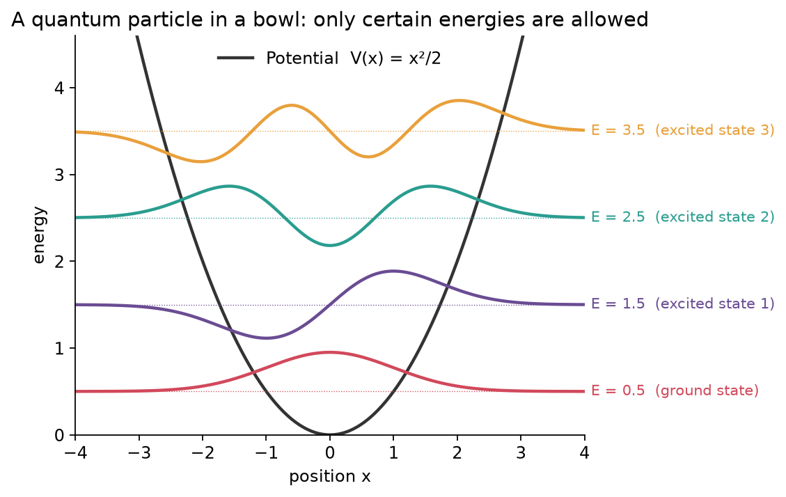
The bottom rung is the floor state. It is the one we need to discover. The Schrödinger equation is the rule that decides which shapes and energies are allowed. For our bowl it’s given as:
I exploit models the place ħ = m = ω = 1. In d dimensions, the lowest-energy and its power eigenstate is thought precisely:
Don’t fret concerning the symbols, which maybe look scary. This is all it’s essential know. H (in physics we name it Hamiltonian) is a recipe that takes a form ψ and returns a brand new form. The allowed states are the particular shapes that come again unchanged, simply multiplied by a quantity E. Mathematicians name this an eigenvalue drawback. The solver should decide each the power (E) and the corresponding wavefunction ψ. Subsequently, one handy strategy is to position the particle inside a sufficiently massive finite field and impose the boundary situation ψ = 0 on the partitions. This synthetic development doesn’t have an effect on the bodily outcome, supplied that the field is chosen massive sufficient. Though the wavefunction formally extends from −∞ to +∞, it decays exponentially at massive distances. Subsequently, for a sufficiently massive field, the wavefunction turns into negligibly small close to the boundaries, and the imposed boundary situations haven’t any vital impact on the calculated power eigenvalues or wavefunctions.
The 2 contenders
Each strategies each attempt to discover the identical curve. However they simply take a look at it in very alternative ways.
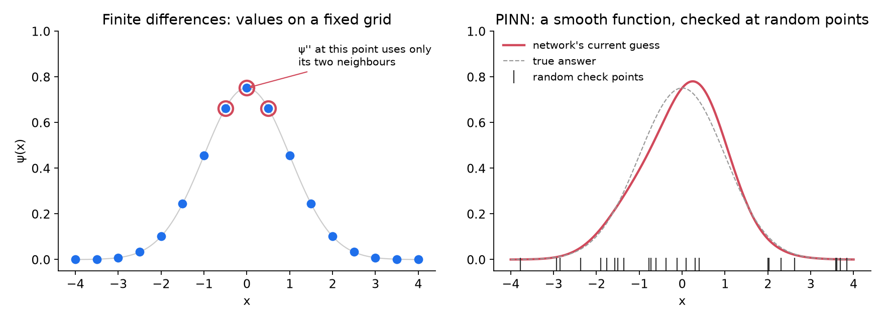
Finite variations technique: I put N factors alongside every axis and change every second spinoff with a easy components that makes use of neighbouring factors. The equation turns into a big sparse matrix, and we use SciPy to search out its lowest eigenvalue.
There is no coaching. The one selection is N. Extra factors imply a greater reply however an even bigger matrix.
The PINN technique: Right here, a small neural community is the wavefunction. You give it a place x, and it returns a quantity ψ(x). At first its guess is random. Coaching improves it step-by-step, like this:
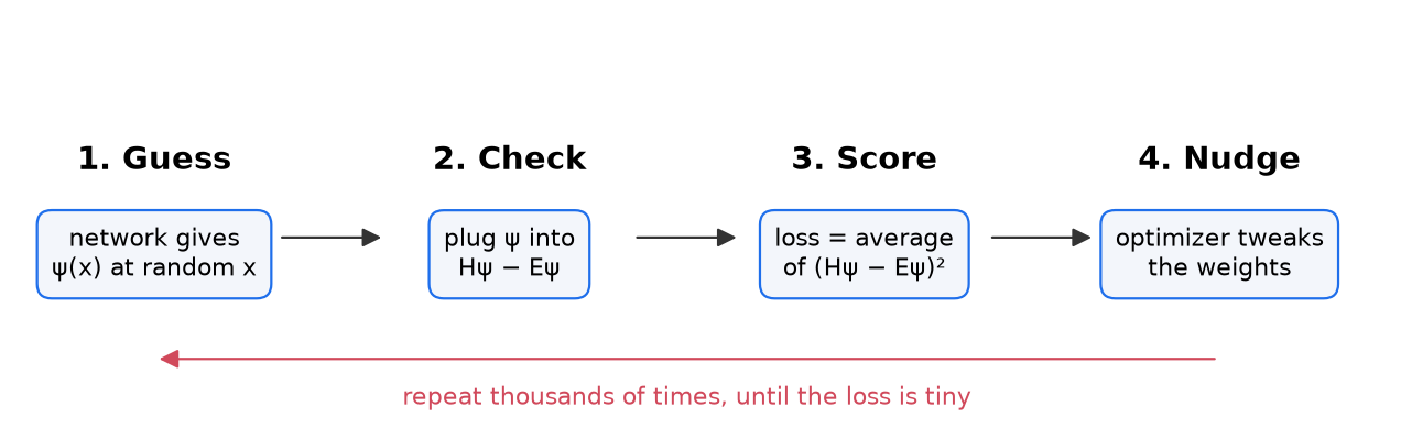
In apply, the loss asks it to fulfill Hψ = Eψ at random factors. However, I compute E from the community itself with the Rayleigh quotient ⟨ψ|H|ψ⟩ / ⟨ψ|ψ⟩, so the power at all times matches the present ψ.
Coaching has two phases. Adam runs first, on contemporary random factors at every step, to get roughly the proper form. Then L-BFGS, a quasi-Newton technique, polishes the outcome on a hard and fast set of factors. That second stage seems to matter quite a bit.
I measured price as CPU time on a laptop computer, not wall-clock time, so background load on the machine would not distort the comparability.
In a single dimension
Each strategies discover the proper floor state. The actual query is how a lot every one prices.
Within the under plot the axes are logarithmic, so every tick is ten occasions larger than the one earlier than. Factors additional left are quicker, and factors decrease down are extra correct. The most effective spot is the bottom-left nook.
|
1D technique |
CPU time |
Vitality error |
Wavefunction error (L₂) |
|---|---|---|---|
|
Finite distinction, N = 100 |
0.8 ms |
4.4 × 10⁻⁴ |
6.5 × 10⁻⁴ |
|
Finite distinction, N = 1600 |
2.5 ms |
1.8 × 10⁻⁶ |
2.6 × 10⁻⁶ |
|
PINN, Adam solely |
~8 s |
~10⁻² |
~4 × 10⁻² |
|
PINN, Adam + L-BFGS |
9 s |
5.7 × 10⁻⁶ |
7.9 × 10⁻⁴ |
Right here two issues are necessary and we should point out.
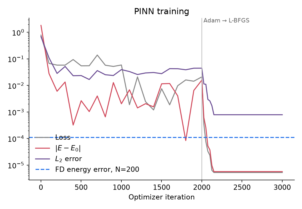
First, L-BFGS rescues the PINN. With Adam alone, the error stalls at just a few p.c. The loss simply bounces round. When L-BFGS takes over, the error drops by an element of about 50 inside just a few hundred iterations. If you wish to take just one tip from this text, take this one.
Why does this occur? Consider coaching as strolling downhill to the bottom level of a panorama. The PINN loss is constructed from second derivatives of the community, which autograd computes by differentiating twice. That makes the panorama stiff or ill-conditioned: it is like an extended, slender canyon, very steep throughout and nearly flat alongside its size. A primary-order technique like Adam solely feels the native slope. So it bounces from wall to wall throughout the canyon and creeps slowly alongside it. That is the noisy plateau within the coaching plot under.
L-BFGS is a quasi-Newton technique. It additionally estimates the curvature, that means how the slope itself adjustments, from its current steps. With that info it may inform which means the canyon runs and take an extended, assured step straight alongside it. For easy bodily issues like this one, that curvature info is near important. Adam is nice for getting roughly into the proper valley shortly however L-BFGS is what helps reache it to the underside.
Second, finite variations nonetheless win simply. They match the PINN’s remaining accuracy in beneath a millisecond. That is roughly ten thousand occasions quicker. And turning N up retains pushing the error down in a predictable means, whereas the PINN ranges off.
The power error can be a lot smaller than the wavefunction error. That is anticipated because the Rayleigh quotient is variational, so a small error in ψ offers a good smaller error in E.
For this 1D drawback, there’s little sensible cause to coach a neural community.
In 5 dimensions
Now let’s make it more durable. I took the identical oscillator in 5 dimensions. The precise reply continues to be identified: E₀ = 2.5.
“5 dimensions” seems like science fiction, but it surely’s very odd in physics. Two particles shifting in 3D house already want six numbers to explain them. Every additional particle provides three extra.
This is the catch for the grid technique. With N factors per axis, a 5D grid has N⁵ factors. With N = 16, that is already 1,000,000 unknowns. With N = 100, it is ten billion. That is known as because the curse of dimensionality.
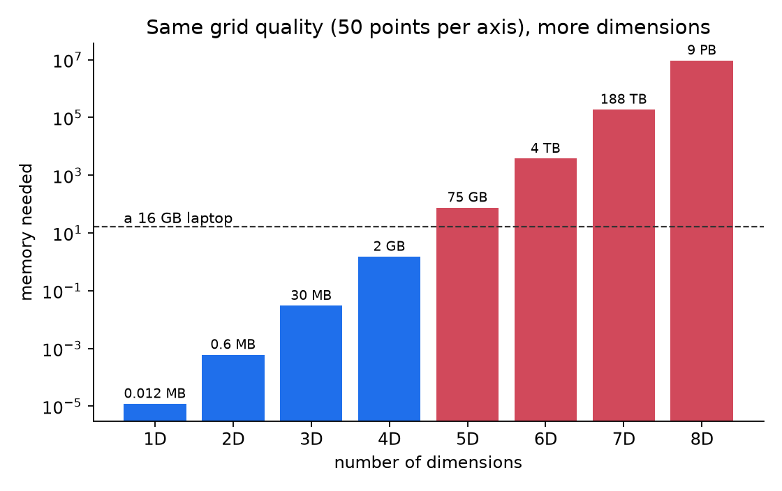
Nonetheless PINN would not want a grid. It samples random factors, so its price grows far more gently with dimension. In concept, that is the place a PINN ought to shine.
Three issues went unsuitable first
My first makes an attempt on the 5D PINN failed. It wanted some fixes, that are value sharing, as they’re straightforward traps.
-
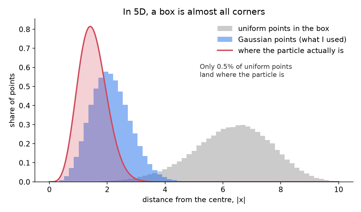
Uniform sampling wastes nearly each level. In 5D, almost all of a field’s quantity lies removed from the centre, the place ψ is mainly zero. So I sampled factors from a Gaussian as an alternative. The determine under reveals why.
-
Significance weights blew up. To show Gaussian samples again into field integrals, you usually weight every level by 1/p(x). In 5D, these weights ranged over about e⁴⁰. Out of 20,000 take a look at factors, solely about 9 actually counted. Subsequently, I educated with out the weights, which continues to be a sound strategy to implement the equation. For testing, I drew factors from |ψ₀|² itself, which retains the weights properly behaved.
-
The community discovered the unsuitable state. This one is shocking. The loss is zero for any eigenstate, not simply the bottom one. My community fortunately settled on E ≈ 3.5, which is the primary excited state. Though it was an ideal answer of the equation, however simply not the one I wished.
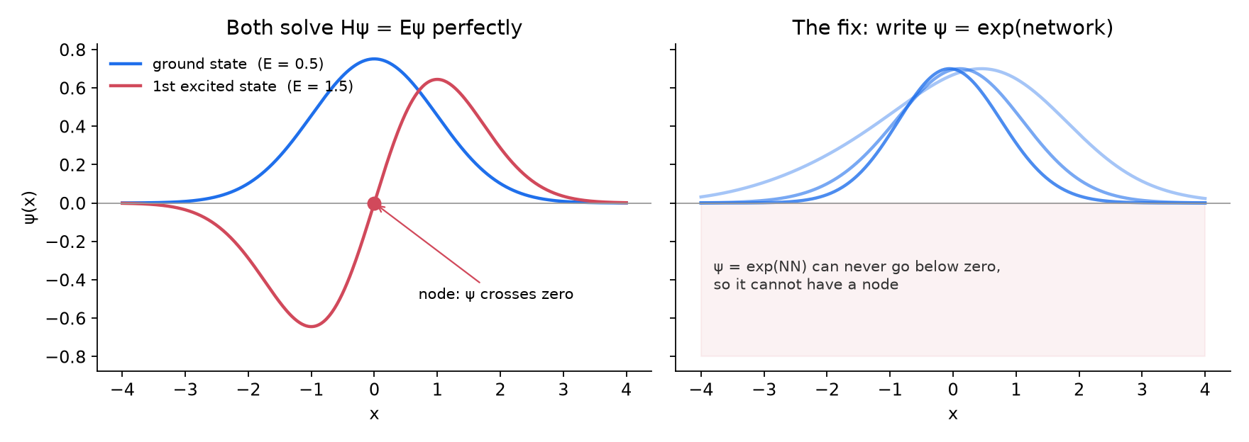
The final repair wants a small piece of physics. A floor state has no nodes, so it by no means adjustments signal. Subsequently, I wrote the community as
The primary issue makes ψ vanish on the partitions. The exponential retains ψ constructive all over the place, so excited states are dominated out. I did not construct within the Gaussian reply. The community nonetheless has to search out the form by itself.
The outcomes
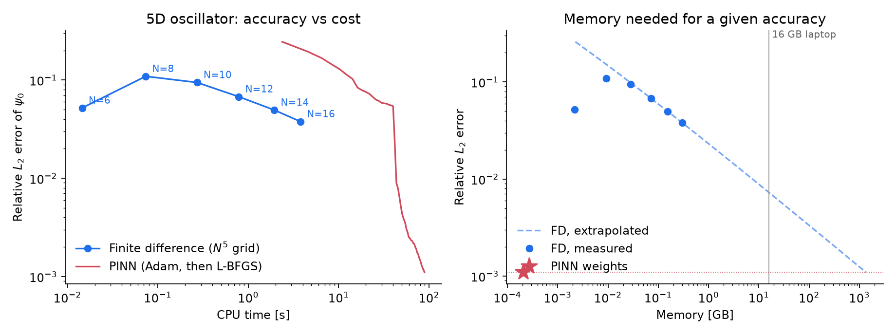
|
5D technique |
Unknowns |
Reminiscence |
CPU time |
Vitality error |
L₂ error |
|---|---|---|---|---|---|
|
Finite distinction, N = 16 |
1.0 million |
0.3 GB |
3.7 s |
5.5 × 10⁻² |
3.8 × 10⁻² |
|
Finite distinction, N ≈ 86 (extrapolated) |
4.7 billion |
~1,400 GB |
— |
— |
~1.1 × 10⁻³ |
|
PINN, Adam + L-BFGS |
~9,000 weights |
< 0.1 GB |
89 s |
6.3 × 10⁻⁵ |
1.1 × 10⁻³ |
Now the image flips.
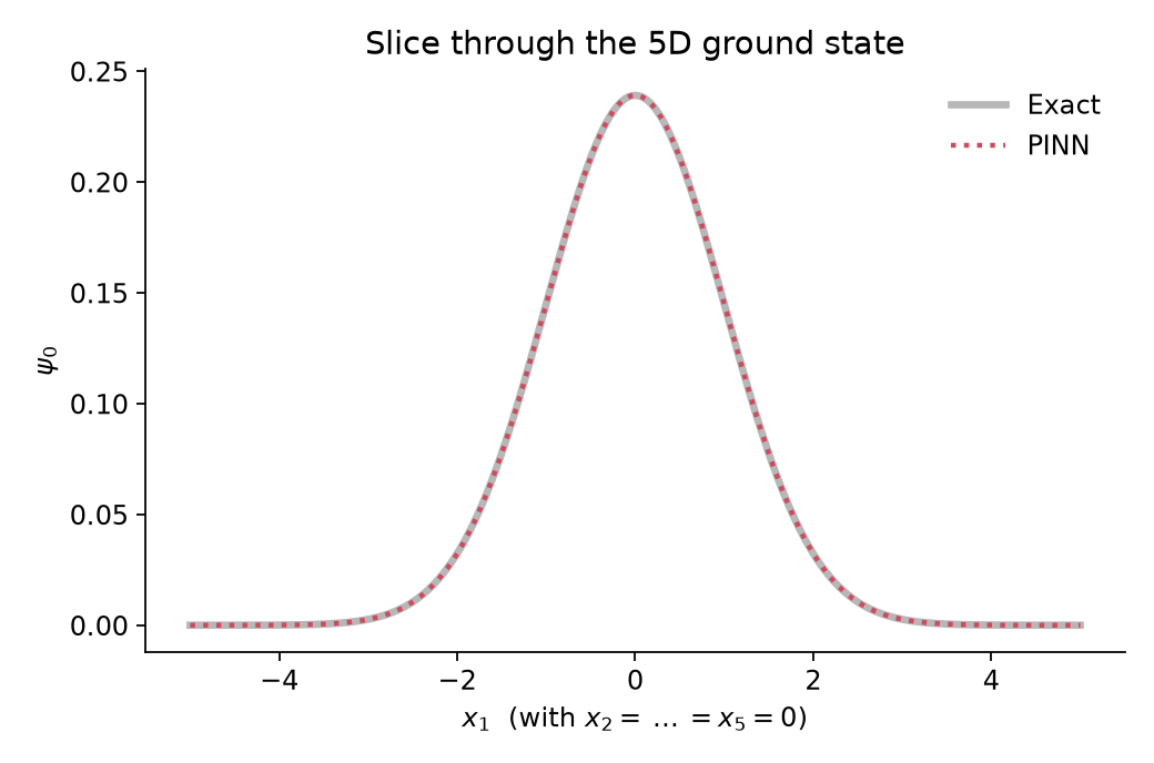
The most important grid I’ve remedy (with N=16) in my laptop computer is with 1,000,000 unknowns and reached about 4% error. The PINN reached about 0.1% in 89 seconds of CPU time. Its power is correct to 5 digits: 2.50006.
For finite distinction technique, the measured grid error falls like h², the place h is the grid spacing. Extending that development, the grid would wish about 86 factors per axis to match the PINN. That is roughly 5 billion unknowns and greater than a terabyte of reminiscence. The PINN suits the entire answer into about 9,000 numbers.
In 1D the grid wins by an element of ten thousand. In 5D the grid cannot even begin.
Is that this a good combat?
Partly. Let me be clear concerning the limits.
The 5D oscillator is separable. It might break up into 5 impartial 1D issues. A wise classical solver that exploits this, utilizing separation of variables, a spectral foundation or tensor strategies, would remedy it nearly precisely in milliseconds. So PINN beats a generic grid solver, not each classical technique. I selected this drawback as a result of its precise reply lets us measure the error actually, not as a result of it is onerous.
The PINN’s actual benefit reveals up when the issue would not separate, for instance with interacting particles or coupled potentials. There, the good classical tips cease working, and also you’re left with grids, foundation units or Monte Carlo. That is why neural-network wavefunctions equivalent to FermiNet and PauliNet have turn into a severe instrument for many-electron methods.
However, the PINN acquired some assist. I used a physics prior (no nodes) and a cautious sampling scheme. With out these, it failed. That is typical. PINNs do not work “out of the field” as typically because the demos counsel.
The grid, alternatively, acquired no assist. I used plain second-order finite variations. The next-order stencil would transfer the grid curve down, but it surely would not change the N⁵ scaling.
So which one is healthier?
It is dependent upon the dimension.
-
In 1, 2 or 3 dimensions, use a classical solver. It is quicker, extra correct and fully predictable. You additionally get many excited states totally free from the identical matrix.
-
In larger dimensions, grids turn into inconceivable, and a PINN or one other neural technique turns into an actual possibility. It nonetheless wants care: good sampling, a second-order optimizer and a few physics constructed into the community.
-
All the time verify for construction first. In case your drawback separates or has symmetry, a classical technique that makes use of it can beat PINN.
Subsequently, my recommendation is easy. Everytime you see a PINN outcome, ask what one of the best classical baseline would have finished with the identical compute. If the paper would not say, run the take a look at your self. In low dimensions it typically takes ten strains of SciPy. Yet one more level is value noting — 5 dimensions are usually not particular right here. The identical argument applies to any sufficiently high-dimensional drawback. I exploit 5 dimensions merely as a handy demonstration of how the computational price of a tensor-product grid grows with dimensionality.
Lastly, the reported CPU occasions ought to be interpreted as consultant moderately than absolute. Precise runtimes can differ relying on the {hardware}, software program surroundings, processor load, and different processes working on the machine. The aim of those timings is due to this fact for example the relative computational price of the 2 approaches, moderately than to offer universally reproducible benchmark occasions.
Strive it your self
All of the code is on GitHub: github.com/Samit1424/pinn-vs-fd-schrodinger. It has two brief Python scripts:
-
schrodinger_pinn_vs_fd.py: the 1D comparability. It takes just a few seconds of CPU time. -
schrodinger_5d.py: the 5D comparability. It might take a few minutes.
Collectively they reproduce each benchmark quantity and outcome plot above. Obtain them and run:
Need an actual problem? Add a coupling time period equivalent to 0.1·x₁²x₂² to the 5D potential so it not separates. (A linear coupling like x₁x₂ will not do as a result of a rotation of the axes separates it once more.) Or attempt a double properly, V(x) = (x² − 1)², in 1D. I might like to listen to the way you get on.
References
-
M. Raissi, P. Perdikaris, G. E. Karniadakis, “Physics-informed neural networks: A deep studying framework for fixing ahead and inverse issues involving nonlinear partial differential equations,” J. Comput. Phys. 378, 686–707 (2019). doi.org/10.1016/j.jcp.2018.10.045
-
N. McGreivy, A. Hakim, “Weak baselines and reporting biases result in overoptimism in machine studying for fluid-related partial differential equations,” Nat. Mach. Intell. 6, 1256–1269 (2024). doi.org/10.1038/s42256-024-00897-5
-
D. J. Griffiths, D. F. Schroeter, Introduction to Quantum Mechanics, third ed., Cambridge College Press (2018), Ch. 2.3. doi.org/10.1017/9781316995433
-
R. J. LeVeque, Finite Distinction Strategies for Strange and Partial Differential Equations, SIAM (2007). doi.org/10.1137/1.9780898717839
-
R. B. Lehoucq, D. C. Sorensen, C. Yang, ARPACK Customers’ Information, SIAM (1998). (Utilized by
scipy.sparse.linalg.eigsh.) doi.org/10.1137/1.9780898719628 -
D. P. Kingma, J. Ba, “Adam: A way for stochastic optimization,” ICLR (2015). arxiv.org/abs/1412.6980
-
D. C. Liu, J. Nocedal, “On the restricted reminiscence BFGS technique for big scale optimization,” Math. Program. 45, 503–528 (1989). doi.org/10.1007/BF01589116
-
P. Rathore, W. Lei, Z. Frangella, L. Lu, M. Udell, “Challenges in coaching PINNs: A loss panorama perspective,” ICML (2024). arxiv.org/abs/2402.01868
-
S. Wang, Y. Teng, P. Perdikaris, “Understanding and mitigating gradient circulation pathologies in physics-informed neural networks,” SIAM J. Sci. Comput. 43, A3055–A3081 (2021). doi.org/10.1137/20M1318043
-
R. Bellman, Dynamic Programming, Princeton College Press (1957).
-
A. S. Krishnapriyan, A. Gholami, S. Zhe, R. M. Kirby, M. W. Mahoney, “Characterizing potential failure modes in physics-informed neural networks,” NeurIPS (2021). arxiv.org/abs/2109.01050
-
D. Pfau, J. S. Spencer, A. G. D. G. Matthews, W. M. C. Foulkes, “Ab initio answer of the many-electron Schrödinger equation with deep neural networks,” Phys. Rev. Analysis 2, 033429 (2020). doi.org/10.1103/PhysRevResearch.2.033429
-
J. Hermann, Z. Schätzle, F. Noé, “Deep-neural-network answer of the digital Schrödinger equation,” Nat. Chem. 12, 891–897 (2020). doi.org/10.1038/s41557-020-0544-y