SIFT is without doubt one of the most generally recognized algorithms in laptop imaginative and prescient. Its core goal consists of detecting object keypoints, producing descriptors for them, and matching the identical objects throughout photos.
Because the title suggests, SIFT is a scale-invariant algorithm, which means that the identical object can seem at totally different scales in a pair of photos, and SIFT will nonetheless be capable to efficiently detect its keypoints.
As well as, SIFT is rotation-invariant, making matching attainable for rotated objects as nicely.
Allow us to take a more in-depth take a look at how SIFT works beneath the hood.
Observe: On this article, we’ll confer with the Laplacian of Gaussian (LoG) as a metamorphosis used for edge detection in photos. If you’re unfamiliar with this method, it’s endorsed that you simply undergo one of many edge detection articles.
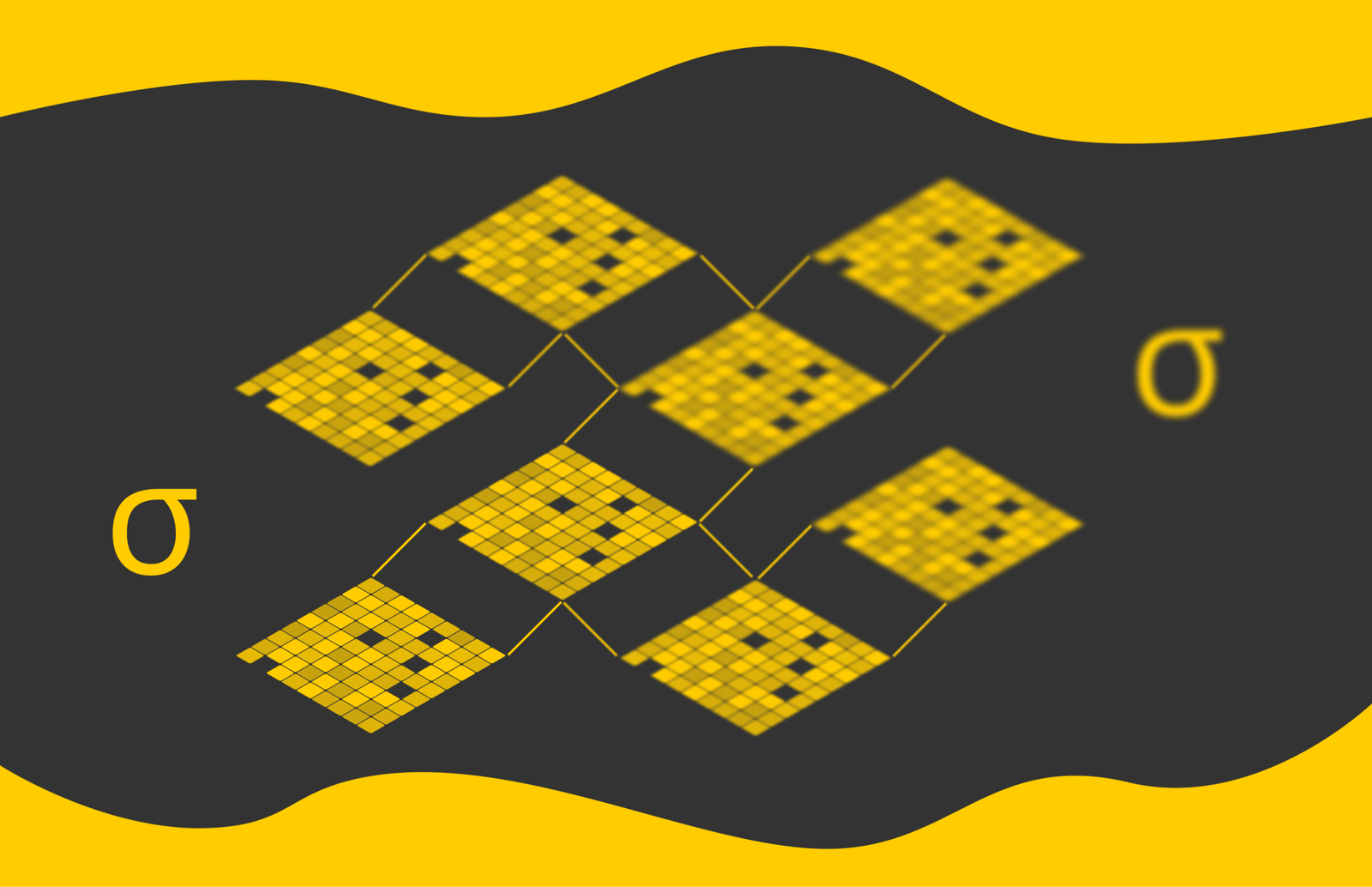
In its workflow, SIFT constructs a number of variations of the unique picture by making use of resize and Gaussian blur transformations.
For simplicity, lets say that I(x, y) is an unique picture. First, with chosen values of okay and σ1, SIFT constructs a number of variations of the unique picture by making use of Gaussian smoothing with totally different normal deviations: σ1, okay⋅σ1, k2⋅σ1, k3⋅σ1, … , the place okay > 1.
This ends in a sequence of photos through which every subsequent picture is barely blurrier than the earlier one. This sequence of photos is known as an octave.
Then SIFT computes the pairwise variations D1, D2, …, Dn between the ensuing photos, generally known as the distinction of Gaussians (DoG). These variations spotlight pixels with excessive depth modifications. After that, the algorithm stacks the Di and tries to seek out native extrema in them. Right here is how it’s executed:
For every level in Di(x, y), SIFT examines its 26 neighbours:
-
8 adjoining factors on Di degree;
-
9 factors straight above Di(x, y) (on the Di+1 degree);
-
9 factors straight beneath Di(x, y) (on the Di-1 degree);
Then one of many following three instances is feasible:
-
If Di(x, y) is larger than all of its 26 neighbouring factors, then SIFT marks it as a most.
-
If Di(x, y) is lower than all 26 neighboring factors, then SIFT marks it at the least;
-
In any other case, the purpose Di(x, y) is skipped.
For simplicity, the purpose Di(x, y) and its 26 neighboring factors could be visualized as a 3x3x3 grid with the middle at Di(x, y). This process permits the identification of the strongest options.
The discovered extrema values symbolize factors of curiosity. In truth, there could be too a lot of them; that’s the reason SIFT applies thresholding or one other operator to retain solely people who symbolize the best modifications.
To account for various scale variations, the identical course of is repeated for an preliminary picture decreased (downsampled) in width and peak by an element of two. Consequently, a brand new octave sequence is constructed with better Gaussian noise utilized to it, having the next σ values: σ2, okay⋅σ2, k2⋅σ1, k3⋅σ2, … , the place σ2 = 2σ1. As earlier than, extrema values are discovered from picture variations utilizing the 3x3x3 grid methodology.
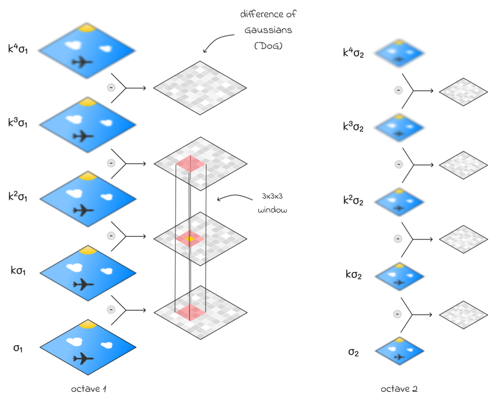
For the third iteration, the picture is downsampled once more (decreased in width and peak by an element of two), and a brand new, blurrier octave is constructed with σ values as σ3, okay⋅σ3, k2⋅σ3, k3⋅σ3, … , the place σ3 = 2σ2 = 4σ1.
The complete course of is repeated for a specified variety of iterations.
We understood tips on how to discover factors of curiosity. Let’s now reply a number of essential inquiries to construct instinct concerning the course of.
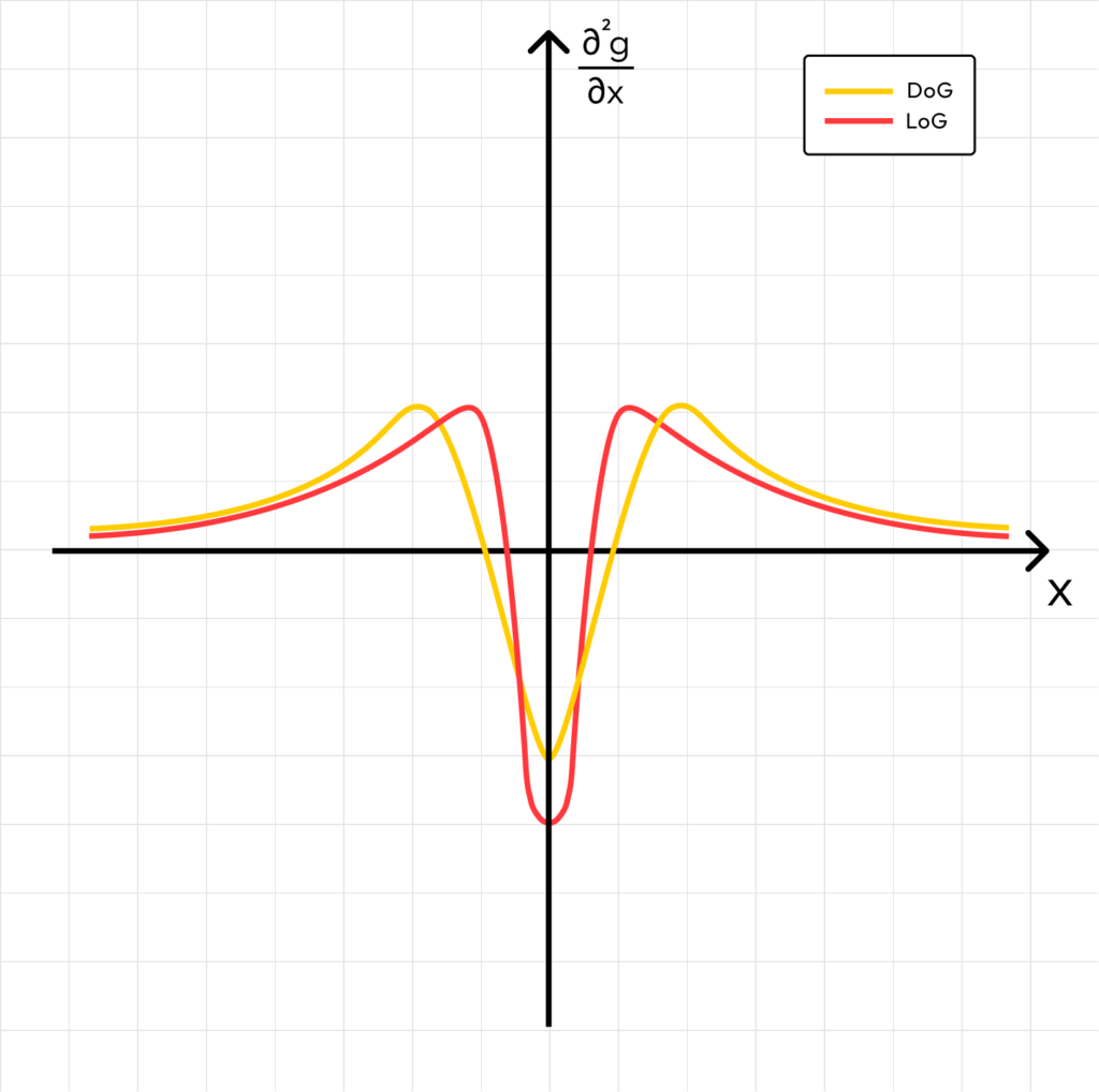
Why DoG as a substitute of LoG?
Up to now, we discovered that the Laplacian of Gaussian (LoG) is a really helpful transformation for figuring out edges in photos. On the similar time, it seems that there exists an excellent approximation for the distinction of two scaled LoGs utilized to the identical picture:
DoG = nkσ – nσ ≈ (okay – 1)σ2 ⋅ ▽2nσ
In truth, calculating DoG utilizing this formulation a number of occasions is way much less computationally costly than making use of the unique LoG formulation every time.
Why assemble a number of DoGs withing a single octave?
Inside a single octave, picture bluriness progressively will increase. The distinction between two consecutive DoGs highlights factors of curiosity throughout scales.
For example, a DoG constructed between a pair of consecutive web photos (on the backside of an octave) makes it a lot simpler to detect smaller options. Nonetheless, for bigger options, that is troublesome. For that cause, we additionally compute a DoG for extra blurred photos (on the prime of an octave), the place smaller options are usually not seen, and the algorithm focuses extra on bigger patches as a substitute.
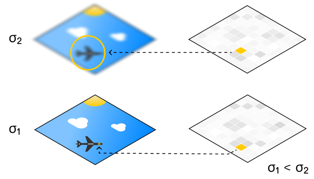
Why to assemble a number of octaves?
It’s clear that as blur will increase, we will detect bigger options. So a pure query arises: why not simply use a single octave, iterating from very small blur ranges to very excessive ones? This fashion, we might detect options of all sizes.
The motivation for the development of a number of octaves lies in two features:
-
As blur will increase, small particulars change into invisible within the picture. So, by way of effectivity, there isn’t any level in holding the total picture decision at greater ranges of blur. Downsampling reduces the variety of pixels by an element of 4, making processing a lot quicker.
-
Approximating very massive Gaussian kernels can accumulate errors, so we should not use excessive values of σ. On the similar time, downsampling could be roughly considered including blur to the unique picture, because it additionally removes superb particulars. On condition that, utilizing greater ranges of blur on the full-resolution picture could be roughly equal to utilizing smaller blur ranges on smaller photos.
Due to this fact, downsampling and octave building present important benefits.
Why a three-dimensional window?
A 3×3 window in a single picture can detect native extrema, however there could also be too many, particularly since we additionally create a number of scaled variations of the picture.
Including a 3rd dimension to the window ensures that the detected factors of curiosity are distinctive not solely on the 2D airplane but in addition throughout totally different scales, making them secure beneath modifications in picture zoom.
If it is unclear why discovering extrema throughout DoG layers yields factors of curiosity, a helpful reminder is that DoG is an approximation of LoG, as outlined above. On the similar time, we defined within the edge detection article that picture edges could be discovered at extrema after making use of the LoG transformation.
After amassing all potential candidate factors, SIFT filters out a few of them. The issue is that even when a given level is an extremum, it will probably nonetheless be noise. To maintain solely probably the most significant ones, SIFT applies a threshold on depth change to take away low-contrast weak candidates.
As soon as curiosity factors are chosen, SIFT tries to assemble descriptor representations for them that can enable these options to be matched throughout totally different photos.
To begin with, detected options throughout totally different DoG layers are mapped to circles of various sizes, the place the upper the σ worth on the DoG layer, the bigger the circle radius. Then, for all pixels within the unique picture inside that circle, gradient instructions are computed.
SIFT then divides the detected area into 4 equal quadrants and constructs a gradient route distribution for every quadrant.
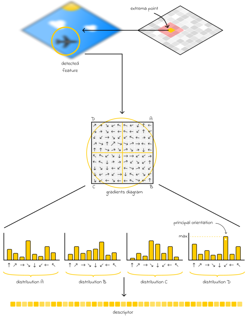
4 constructed distributions are then transformed right into a 128-dimensional vector, which is used as a function descriptor for the initially detected function.
For reference, SIFT offers sturdy inner mechanisms that enable it to deal with conditions through which a detected function has fewer than 128 pixels. SIFT nonetheless permits computing a 128-dimensional vector descriptor by making an allowance for data from neighboring pixels as nicely.
A typical case in real-world issues is when the identical object seems in two photos rotated by totally different quantities. To account for rotation appropriately, SIFT additionally makes use of extra details about the principal orientation of the gradient, which is just the commonest gradient route within the distribution. From a rotational perspective, this enables defining the start line of the thing, enabling right mapping with others and serving to keep away from false-positive matches. These features assure the rotational invariance of the SIFT algorithm.
Evaluating SIFT descriptors
SIFT descriptors are vectors that may be in contrast numerically to find out how related they’re to one another. The most typical use case for descriptor comparability is figuring out whether or not the focal point for which the descriptor is computed is similar throughout a pair of photos.
L2-distance is a typical alternative for descriptor comparability:
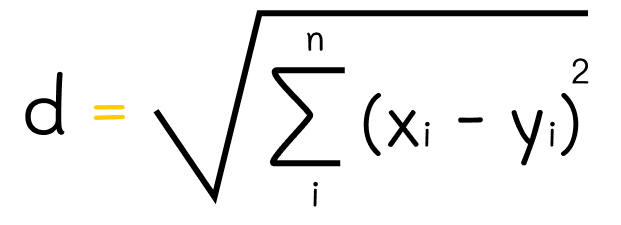
The decrease the L2-distance, the higher the match between two factors. If the L2-distance is 0, the match is ideal.
One other helpful metric is histogram intersection:
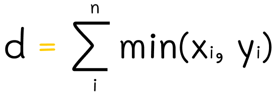
Right here, the formulation iterates by way of every vector part and finds the minimal of two values, which is equal to how nicely a selected aggregated gradient route is current in each options. On this case, a better metric worth corresponds to raised matching outcomes.
Usually, the identical objects throughout totally different photos are anticipated to have many matches, making it attainable to acknowledge their id.
OpenCV offers an implementation of the SIFT algorithm. To create a SIFT object, the cv2.create_SIFT() methodology must be referred to as. In line with the SIFT documentation, a number of parameters could be specified:
-
nfeatures: the variety of finest options to retain. The options are ranked by their scores (measured in SIFT algorithm).
-
nOctaveLayers: the variety of layers in every octave. 3 is the worth used within the paper.
-
contrastThreshold: the distinction threshold used to filter out weak options in low-contrast areas. The bigger the brink, the much less options are produced by the detector.
-
edgeThreshold: the brink used to filter out edge-like options. The bigger the edgeThreshold, the much less options are filtered out (extra options are retained).
-
sigma: the sigma of the Gaussian utilized to the enter picture on the first octave.
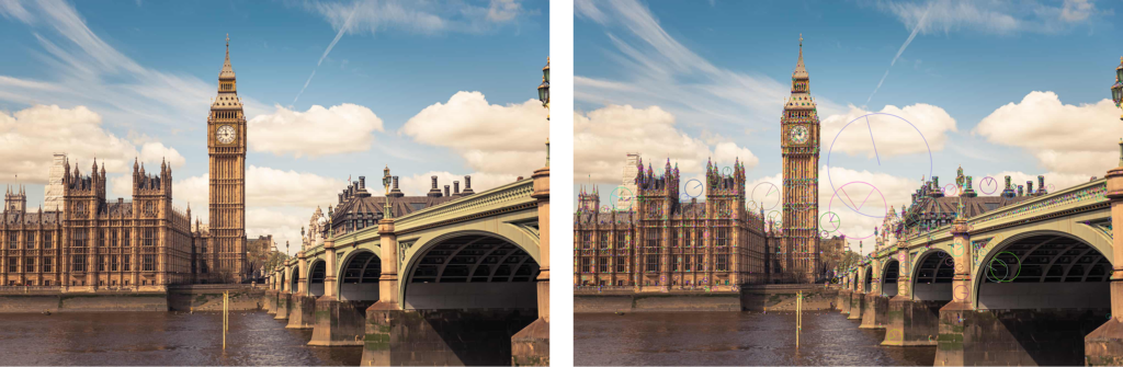
Aside from the usual algorithm, we will simply visualize detected options on the picture utilizing the straightforward code snippet beneath.
Here’s what the consequence seems like:

In actuality, for extra advanced real-life photos, the variety of detected options could be a lot greater. Under is one other instance:
SIFT has a variety of functions. Let’s take a look at them.
Picture matching
As talked about earlier than, function descriptors can be utilized for picture matching. Let’s take a look at one instance utilizing the next picture pair:

First, we’ll learn a pair of photos. Keep in mind that earlier than feeding them to SIFT, they should be transformed to grayscale.
We then compute descriptors for every picture.
Subsequent, we’ll make the most of BFMMatcher, or Brute-Power Matcher. This algorithm compares each descriptor within the first picture with each descriptor within the second picture, figuring out the closest pairs based mostly on the chosen distance measure. In our code, we’re utilizing the L2-distance.
By calling the knnMatch() methodology, we move all descriptors from each photos and set okay = 2, which specifies how most of the prime okay closest matches are returned for every descriptor.
The objective of setting the parameter okay to a worth better than 1 is to take away much less related matches by utilizing Lowe’s ratio check.
The check consists of figuring out how good one of the best match is in contrast with the second-best match.
For example, within the code beneath, we filter solely good matches the place the gap to one of the best match is lower than the gap to the second-best match, scaled by RATIO = 0.75.
Because it seems, we will nonetheless find yourself with too many matches, so we hold solely one of the best MAX_MATCHES = 50.
Lastly, we will draw matches utilizing the cv2.drawMatches() operate.
Right here is the consequence:

As we will see, SIFT did its job very nicely! It appropriately matched the primary objects in each scenes. A really fascinating remark is that SIFT efficiently preserved scale and rotation invariance!
For instance, we will see that the airplane was scaled and rotated in a different way in every scene. Regardless of this, SIFT produced very related descriptors for every airplane function.
Object detection
One other SIFT software is object detection. With an object template, we will carry out picture matching in the identical method as above to seek for that object in a picture.
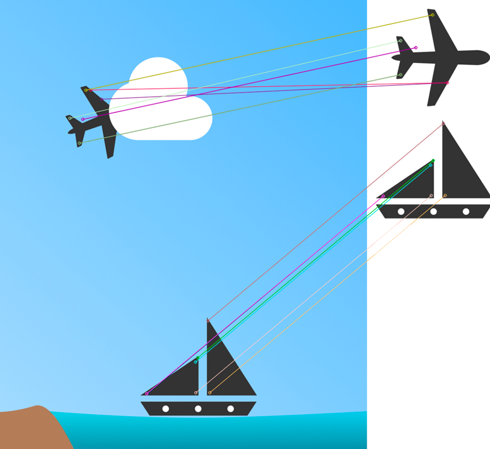
An ideal side of SIFT is that it tends to be sturdy in opposition to occlusions. If part of an object is overlaid by one other object, SIFT can nonetheless detect the seen options and match them efficiently.
As soon as function matching is full, extra postprocessing strategies could be utilized to extract the thing’s contour and decide its exact location within the picture.
It’s value noting that SIFT can generally produce false-positive matches, as proven within the picture above. We are able to clearly see a purple line connecting the airplane’s left wing within the scene on the left to its endpoint within the object template on the proper, the place it matches some extent on the proper wing.
Such conditions can happen occasionally, and normally, they don’t have a strongly adverse influence. Relying on the duty, postprocessing algorithms (e.g., RANSAC) can eradicate false-positive matches if there are usually not too many.
Picture stitching
Picture stitching is the duty of merging photographic photos taken from a single viewpoint which have overlapping areas right into a single high-resolution picture (a panorama). Picture stitching could be elegantly solved with function matching, perspective warping, and geometric transformations.
To do this, it’s mandatory to know homography, which we’ll cowl in one of many subsequent articles.
3D-reconstruction?
Whereas SIFT works very nicely for flat and 2D objects, it’s sadly not appropriate alone for matching 3D objects.
Nonetheless, SIFT is used as one of many core steps in different 3D reconstruction algorithms (e.g., COLMAP). It permits matching factors throughout photos, from which the entire 3D scene is then constructed.
SIFT is a extremely versatile algorithm for function matching, notable for its capability to match options whereas sustaining rotation and scale invariance.
As we noticed, SIFT can resolve a variety of issues in laptop imaginative and prescient. Picture matching, object detection, and picture stitching are among the many hottest SIFT functions. In additional subtle issues, SIFT is usually used as a robust spine for function matching, which is then processed in a different way relying on the issue itself.
All photos except in any other case famous are by the writer.