
# Introduction
Coaching a machine studying mannequin and observing the loss lower is a sense of progress, till the validation accuracy reaches a plateau or the loss begins to spike, and also you’re unsure what brought on it. At that time, most individuals add extra logging or begin tuning hyperparameters, hoping one thing modifications. What most analysts skip at this stage is precise visibility into what is going on contained in the mannequin throughout coaching. Visible debugging instruments can present helpful insights at this stage.
On this article, we cowl three subjects: what to visualise throughout coaching (gradients, losses, and embeddings), the instruments that present these visualizations (TensorBoard and its essential alternate options), and the strategies to seize mannequin computations instantly utilizing hooks and breakpoints.
# Visualizing Gradients, Losses, and Embeddings
// Loss Curves
When coaching a mannequin, the loss curve is normally the very first thing to examine. When each the coaching loss and validation loss decline and stay shut, it signifies that the coaching is progressing nicely. When validation loss begins rising whereas coaching loss retains falling, the mannequin is overfitting. When each curves plateau early, the mannequin is not studying, which generally signifies an issue with the information or studying price.
As well as, gradient move can also be necessary. The vanishing gradient drawback could manifest in follow if the loss curves lower easily however too slowly, indicating that gradients are too small by the point they attain early layers.
The plot proven under simulates a typical overfitting sample. Each losses lower collectively for the primary ten epochs, after which the validation loss begins growing whereas the coaching loss retains falling.
The purple dotted line marks the place the divergence begins: in an actual run, that is the purpose to start out investigating regularization or early stopping.
import torch
import torch.nn as nn
import matplotlib.pyplot as plt

mannequin = nn.Sequential(nn.Linear(16, 16), nn.Tanh(),
                      nn.Linear(16, 16), nn.Tanh(),
                      nn.Linear(16, 1))

grad_magnitudes = {}

def grad_hook(title):
    def hook(module, grad_input, grad_output):
        grad_magnitudes[name] = grad_output[0].abs().imply().merchandise()
    return hook

for i, layer in enumerate(mannequin):
    layer.register_backward_hook(grad_hook(f"Layer {i}"))

output = mannequin(torch.randn(32, 16))
output.imply().backward()

plt.bar(grad_magnitudes.keys(), grad_magnitudes.values())
plt.title("Imply Gradient Magnitude per Layer")
plt.ylabel("Imply |gradient|")
plt.xticks(rotation=15)
plt.tight_layout()
plt.present()
It outputs:
// Uncooked Gradient Magnitudes
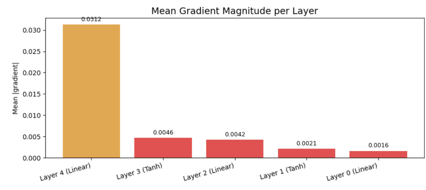
Layer 4 (Linear): 0.031250
Layer 3 (Tanh): 0.004646
Layer 2 (Linear): 0.004241
Layer 1 (Tanh): 0.002126
Layer 0 (Linear): 0.001631
The chart reads proper to left: Layer 4 represents the output layer, and Layer 0 is the primary. The output layer will get a gradient of 0.031, however by the point it reaches Layer 0, that quantity has dropped to 0.0016 — roughly 20 instances smaller.
The purple bar that seems on every of the primary three layers signifies that gradients are already within the danger zone earlier than they ever attain the beginning of the community. In an actual coaching run on a deeper mannequin, these preliminary layers would alter their weights so slowly that they’d hardly be taught something.
It is a sensible instance of the vanishing gradient drawback: the early layers are silently undertraining, which may’t be seen with out this type of plot.
// Gradient Visualization
Plotting gradient magnitudes layer by layer throughout coaching provides a direct view of whether or not gradients are reaching the early elements of the community with appreciable values. In deep fashions, gradients could vanish as they transfer backward via layers. The gradient worth histograms for every layer, recorded throughout coaching, can reveal this sample and assist us establish the difficulty early on.
PyTorch‘s register_backward_hook operate permits us to acquire gradient tensors from any layer with out modifying the coaching loop. We join a hook to a module, which prompts throughout every backward move, sending the gradient tensors to a specified callback.
The histogram under exhibits the entire distribution of gradient values for every layer after one backward move. Every subplot represents a single layer, ordered from the preliminary layer to the ultimate one.
The code for this may be discovered right here.
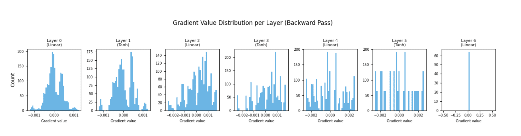
What we’re searching for in a wholesome community is histograms throughout layers with roughly related spreads.
If the early layers present a really slim, spike-like distribution centered tightly on zero, that may very well be a purple flag indicating vanishing gradients.
The gradients nonetheless exist, however they’re so small they carry virtually no studying data. This visualization might help us catch this sample after the primary few batches, fairly than after a full coaching run.
// Embeddings
When a mannequin maps inputs to a discovered illustration, visualizing that illustration tells us whether or not the mannequin is separating the information as we would anticipate. The most typical method is to take the embeddings from a skilled (or partially skilled) mannequin, scale back their dimensionality utilizing t-SNE or UMAP, and plot them with class labels as colours.
If the courses are tight and well-separated, which means the mannequin has discovered helpful separation. Overlapping courses imply the mannequin hasn’t separated the ideas but. This step is beneficial for debugging fashions skilled on textual content or photographs earlier than including the ultimate classification layer.
# TensorBoard and Its Alternate options
// TensorBoard
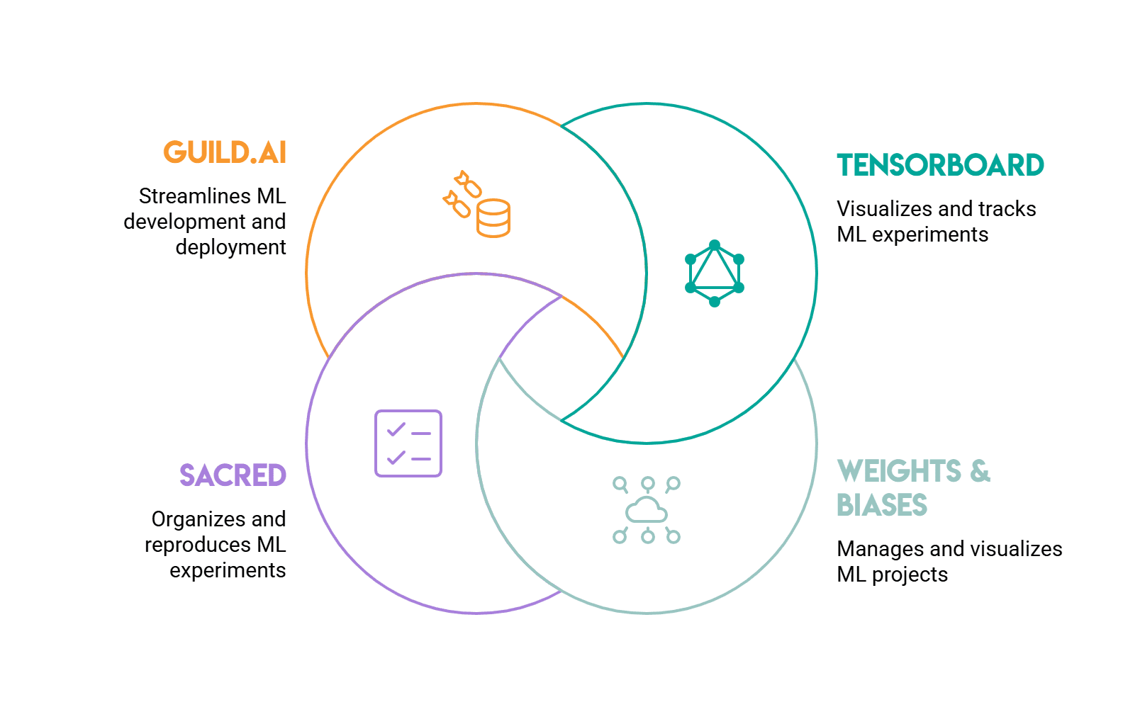
TensorBoard is your normal place to begin. Initially constructed for TensorFlow, it really works with PyTorch via torch.utils.tensorboard. Knowledge will be logged via a SummaryWriter object, and you’ll view the leads to a browser tab. It handles scalars (loss, accuracy), histograms (weight and gradient distributions), photographs, and an embedding projector for visualizing high-dimensional representations.
The principle limitation is its locality. Sharing your outcomes with a crew means organising shared storage for log information or utilizing TensorBoard.dev, which has limits on what it helps.
// Weights & Biases
Weights & Biases (W&B) is what most machine studying groups use for collaboration or extra detailed monitoring.
Setup is finished with two traces: wandb.init() at first of a run and wandb.log() contained in the coaching loop. All the pieces syncs to a cloud dashboard mechanically, and runs are grouped by mission, making experiment comparability simple.
Test the code snippet under:
import wandb

wandb.init(mission="my-model", config={"lr": 0.001, "epochs": 20, "batch_size": 32})

for epoch in vary(wandb.config.epochs):
    train_loss = 1 / (1 + 0.3 * epoch)   # simulated
    val_loss   = train_loss + max(0, 0.04 * (epoch - 10))  # simulated
    wandb.log({"epoch": epoch, "train_loss": train_loss, "val_loss": val_loss})

wandb.end()
As soon as the run finishes, the logged metrics will be seen within the W&B dashboard, alongside the configuration that produced them. Evaluating two runs with totally different parameters can simply be performed by deciding on them within the interface, with no guide log parsing wanted.
W&B additionally helps hyperparameter sweeps with built-in visualization, exhibiting which hyperparameters affected the result essentially the most.
System metrics like GPU utilization and reminiscence utilization are additionally logged mechanically. For groups operating many experiments in parallel, the shared workspace removes a number of the guide overhead of retaining monitor of what was tried.
// Sacred
Sacred takes a special method. It focuses on reproducibility fairly than visualization. We annotate a coaching script with Sacred’s experiment decorator, which information your complete configuration, any modifications made throughout runtime, and all recorded metrics in a database (normally MongoDB). This manner, every run and its exact settings flip right into a everlasting file.
For the visualization half, Sacred pairs with front-ends like Omniboard or Sacredboard. This provides complexity in comparison with TensorBoard or W&B, however the energy is auditability: any run from the previous will be reproduced precisely because it was configured.
// Guild.ai
Guild.ai works from the command line and would not require you to alter the coaching code. We run a coaching script via Guild utilizing guild run prepare.py, which information all of the logs produced by the script together with any output information, linking them to that specific run. Metrics and run comparisons can be found via Guild’s command-line interface (CLI) or its native UI.
This framework is an effective selection when working with current scripts or third-party code that we choose to not modify. It gives fewer options than W&B, however the setup value can also be decrease.
# Utilizing Breakpoints and Hooks for Machine Studying Computations
// Ahead and Backward Hooks
PyTorch’s hook system lets us intercept computations at any level in a mannequin’s ahead or backward move. The register_forward_hook operate attaches a callback to any layer, and it fires each time that layer processes a batch. The callback captures the layer’s enter and output tensors, which we will then log, examine for NaN values, or plot.
The register_backward_hook operate does the identical for the backward move, giving us entry to the gradient tensors flowing via every layer. Collectively, these two hooks cowl most of what we would need to examine throughout coaching with out modifying the mannequin definition or the coaching loop.
A sensible software is the detection of NaN values. A ahead hook that evaluates tensor.isnan().any() at each layer’s output detects numerical instability instantly, stopping it from spreading and damaging the remainder of the coaching.
This is a minimal working instance, utilizing a three-layer mannequin with a hook connected to every layer:
import torch
import torch.nn as nn

mannequin = nn.Sequential(nn.Linear(8, 16), nn.ReLU(), nn.Linear(16, 4))

def nan_hook(layer, enter, output):
    if output.isnan().any():
        print(f"[NaN detected] Layer: {layer.__class__.__name__}")
    else:
        print(f"[Clean] Layer: {layer.__class__.__name__}, output form: {tuple(output.form)}")

for layer in mannequin:
    layer.register_forward_hook(nan_hook)

print("--- Regular enter ---")
mannequin(torch.randn(2, 8))

print("n--- Corrupted enter ---")
bad_input = torch.randn(2, 8)
bad_input[0, 3] = float('nan')
mannequin(bad_input)
Anticipated output when run:
--- Regular enter ---

[Clean] Layer: Linear, output form: (2, 16)
[Clean] Layer: ReLU, output form: (2, 16)
[Clean] Layer: Linear, output form: (2, 4)

--- Corrupted enter ---

[NaN detected] Layer: Linear
[NaN detected] Layer: ReLU
[NaN detected] Layer: Linear
On this instance, the hook checks the output tensor after every layer fires and experiences whether or not it is clear or corrupted.
Working it twice — as soon as with regular enter and as soon as with a single NaN injected — demonstrates how instability propagates via the community, layer by layer.
// Debugger Breakpoints
Commonplace Python debuggers work effective inside coaching loops.
Dropping import pdb; pdb.set_trace() at any level pauses execution and brings up an interactive immediate that enables us to look at tensor shapes, confirm that knowledge preprocessing hasn’t produced sudden values, and manually step via the ahead move.
Most machine studying improvement environments — VSCode and PyCharm each — allow us to set breakpoints graphically and examine tensors in a devoted pane, providing a faster various to the terminal-based pdb interface.
Nonetheless, breakpoints are notably worthwhile through the preliminary one or two batches, as we verify that the information, mannequin, and loss operate are working correctly earlier than beginning an entire coaching run.
# Conclusion
Coaching a mannequin with out visualizing what’s taking place inside means deciphering signs fairly than the precise causes.
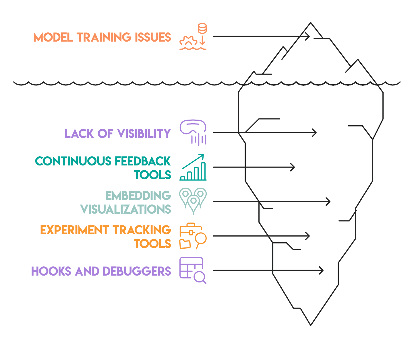
When coaching a mannequin, whether or not the loss curve plateaus early, gradients vanish, or embeddings do not separate, with out the proper instrumentation, none of those components announce themselves clearly.
The instruments coated on this article function at totally different ranges. Loss curves and gradient histograms give steady suggestions throughout coaching, catching issues like overfitting or vanishing gradients earlier than they compound and break your framework.
Embedding visualizations reveal whether or not the mannequin is studying a superb separation from the information. TensorBoard, W&B, Sacred, and Guild.ai every deal with the logging and monitoring aspect in a different way, however all of them serve the identical objective: making experiment historical past searchable and comparable fairly than scattered. Lastly, hooks and debuggers go one step additional and allow you to pause and examine the precise tensors flowing via the community at any layer.
Nonetheless, these instruments cannot repair a damaged mannequin on their very own. What they do is shorten the gap between one thing going improper and understanding why — which is normally many of the work.
Nate Rosidi is an information scientist and in product technique. He is additionally an adjunct professor instructing analytics, and is the founding father of StrataScratch, a platform serving to knowledge scientists put together for his or her interviews with actual interview questions from prime firms. Nate writes on the newest traits within the profession market, provides interview recommendation, shares knowledge science tasks, and covers all the things SQL.