Optimizing AI Agent Planning with Operations Analysis and Information Science

to massive enterprises, an increasing number of organizations are embracing AI brokers and adopting multi-agent architectures to ship dependable, scalable, and manageable options. AI agent and LLM prices can shortly spiral with out cautious administration. On this submit, we are going to uncover a number of agent planning and value optimization enterprise issues and body them as operations analysis options by means of the lens of knowledge science. If you’re considering studying extra about Agent Planning and Agentic AI, take a look at my article on “Easy methods to Construct Your Personal Agentic AI System Utilizing CrewAI“.

What’s Optimization in Operations Analysis?

Operations analysis leverages mathematical fashions and optimization to search out the very best determination underneath sensible constraints. It’s the spine of prescriptive analytics, which transforms predictive insights to actions which can be crucial to determination making. Framing a real-world scenario into an summary mathematical mannequin is the important thing to fixing any operations analysis drawback.

A easy but broadly talked about instance of operations analysis is the linear programming drawback, the place we attempt to discover values of x and y that maximize a linear equation (e.g. 2x + 4y), topic to the constraints x ≥ 0 and y ≥ 0. Operations analysis issues usually embody the next key elements:

1. Choice Variables: The variables to be decided.
2. Constraints: The true-world limitations on assets or necessities.
3. Targets: The purpose to be maximized or minimized.

Easy methods to Optimize Agent Value and Useful resource Allocation

AI agent planning entails making useful resource allocation choices inside an organization’s funds whereas nonetheless attaining the very best outcomes, which makes it a robust match for operations analysis eventualities. We are able to map the core elements above to agent price optimization and useful resource planning use instances.

• Choice Variables: Brokers assign to duties or initiatives
• Constraints: funds, response time, token
• Targets: reduce prices, maximize return on funding

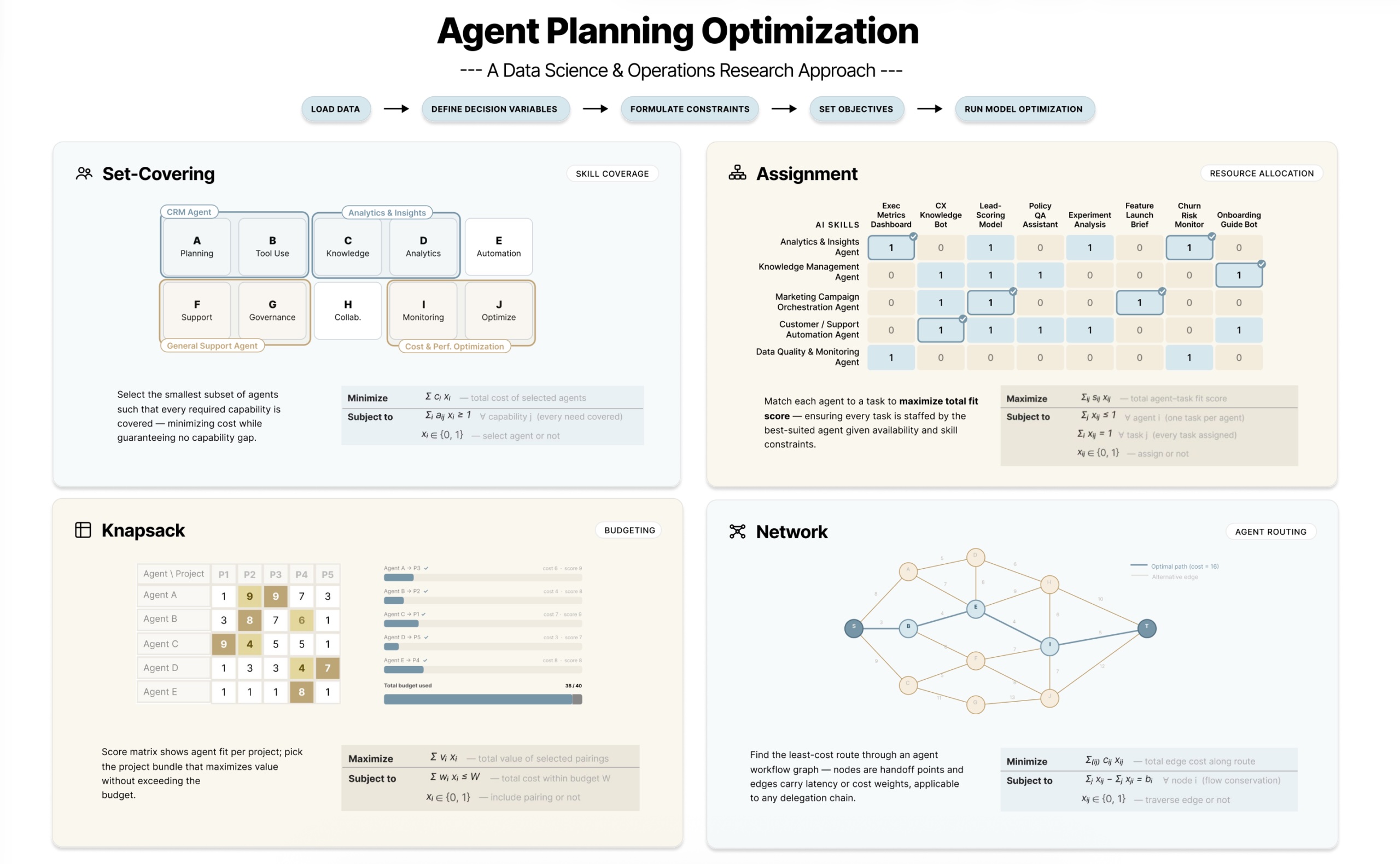
We’ll use 4 most traditional optimization patterns to deal with widespread agent planning eventualities:

• Set-Protecting Drawback: Select the smallest set of brokers to cowl all required duties, expertise, or enterprise capabilities, with the target of minimizing price with out leaving gaps in functionality.
• Project Drawback: Resolve which agent ought to deal with every mission, with the purpose of maximizing total output worth.
• Knapsack Drawback: Choose the very best bundle of brokers underneath a hard and fast funds, to maximise whole output tokens.
• Community Drawback: Design workflows throughout a community of brokers to fulfill division and person calls for on the lowest price underneath capability constraints.

To make this extra sensible, we are going to stroll by means of 4 examples in Python utilizing the Gurobi library. Gurobi is an enterprise-grade mathematical optimization solver that helps many drawback varieties, together with linear programming and mixed-integer programming. It’s usually used because the “solver engine” behind operations analysis purposes as a result of it could actually deal with large-scale fashions effectively and gives sturdy APIs, together with Python, for outlining determination variables, constraints, and goal capabilities. Gurobi lets information scientists deal with modeling reasonably than implementing customized optimization algorithms. Please notice that this text will not be affiliated with Gurobi, and all functionalities talked about right here could be achieved utilizing the free license. All datasets proven on this mission are artificial and are used to display a proof of idea.

1. Set-Protecting Drawback – Agent Ability Protection

Set-covering is a basic optimization drawback refers back to the drawback of selecting the smallest variety of choices in order that each required merchandise is roofed at the least as soon as. A typical AI agent cost-optimization situation that matches the set-covering drawback is ability protection, the place we goal to determine the minimal variety of brokers wanted to cowl the basic expertise required to help the corporate’s every day operations.

Drawback Assertion: The corporate needs to embed brokers into every day operations and canopy the 9 ability areas listed within the “Ability Space” desk under. Every agent prices $20k to construct and makes a speciality of a definite set of expertise as proven within the “Agent Ability” desk. How can the corporate reduce the overall price of constructing brokers whereas nonetheless protecting each space?

Ability Space

Agent Ability

Implementation

We are able to body it as an optimization drawback that follows the set-covering sample and clear up it utilizing Gurobi library, outlined by following key elements — information, mannequin, variables, constraints and goals.

• Information: load the information for expertise, brokers and agent prices (which is 20k every agent)

## information
expertise = information["skills"]
brokers = information["agents"]
agent_skills = information["agent_skills"]
agent_costs = {i: 20 for i in brokers}

• Mannequin: Create the Gurobi mannequin with a reputation “Set Protecting”. If you happen to haven’t put in gurobipy but, run the command

## mannequin
import gurobipy as gp
mannequin = gp.Mannequin("Set Protecting")

• Variables: The choice variables are binary variables related to each agent, with a decrease sure of 0 and an higher sure of 1 to point whether or not an agent is chosen. Gurobi affords a spread of preset variable varieties, together with GRB.BINARY, GRB.INTEGER, and GRB.CONTINUOUS, and many others.

## variables
X = mannequin.addVars(brokers, lb=0, ub=1, vtype=GRB.BINARY, title="x")

• Constraints: For every ability space, sum of all chosen brokers with that ability needs to be greater than 1, making certain that we’ve at the least one agent to cowl the ability space. We use the summation operate gp.quicksum so as to add constraints utilizing weighted sum after which use nested loop expressions to iterate by means of 9 ability areas.

## constraints: for every ability in expertise, sum of brokers with that ability ≥ 1
for j in expertise:
    mannequin.addConstr(
        gp.quicksum(X[i] for i in brokers if j in agent_skills[i]) >= 1,
        title=f'{j}_area_constr'
    )

• Goal: Reduce the overall price of chosen brokers, calculated because the weighted sum of every agent’s price multiplied by the choice variable indicating whether or not that agent is chosen.

## goals: reduce sum of brokers chosen
mannequin.setObjective(
    gp.quicksum(agent_costs[i] * X[i] for i in brokers),
    GRB.MINIMIZE
)

Lastly, we run the mannequin optimization utilizing mannequin.optimize().

Enterprise Affect

On this part, we first interpret the mannequin’s optimum output after which estimate the influence of creating choices based mostly on that optimum output versus making random decisions. In a enterprise setting, this helps leaders allocate funds successfully by figuring out which brokers to construct, deploy, or retire.

Optimum Outcome

mannequin.ObjVal prints out the optimum goal worth. For every binary determination variable, we use X[i].X > 0.5 to print out the chosen brokers.

print(f"Whole brokers chosen: {spherical(mannequin.ObjVal, 4)}")
for i in brokers:
    if X[i].X > 0.5:
        print(f"Agent {i} chosen.")

Alternatively, Claude Code suggests me the next snippet to show the mannequin output in a structured method.

print("================ Set-Protecting: Ability Protection ================")
if mannequin.Standing == GRB.OPTIMAL:
    chosen = [i for i in agents if X[i].X > 0.5]
    print(f"Minimal brokers wanted : {len(chosen)}")
    print(f"Whole price            : ${mannequin.ObjVal:.0f}ok")
    print("nSelected brokers:")
    for agent in chosen:
        coated = ", ".be part of(
            f"{s}({skill_labels[s]})" for s in agent_skills[agent]
        )
        print(f"  - {agent}  [{covered}]")
else:
    print("No optimum answer discovered.")

Output under exhibits that the optimum agent planning is to pick out 4 brokers (Normal Help Agent, Entry & Permissions Agent, CRM Agent and Value & Efficiency Optimization Agent) to cowl all expertise with $80k funds spend.

================ Set-Protecting: Ability Protection ================
Minimal brokers wanted : 4
Whole price            : $80k

Chosen brokers:
  - Normal Help Agent  [F(Support), C(Knowledge), H(Collaboration)]
  - Entry & Permissions Agent  [F(Support), E(Automation), G(Governance)]
  - CRM / Relationship Administration Agent  [A(Planning), B(Tool Use), C(Knowledge)]
  - Value & Efficiency Optimization Agent  [D(Analytics), I(Monitoring), J(Optimization)]

Simulations

We then simulated random choices and in contrast them with the optimum final result. As proven under, we generated 500 possible agent choices (blue histogram) with prices starting from $80k to $200k and a mean price of $134.6k (blue dotted line). This implies the optimization helps the enterprise to cut back the price by ($134.6k − $80k)/$134.6 = 40.6% on common.

──────────────────────────────────────────────────
  Set Protecting — Ability Protection
──────────────────────────────────────────────────
  Minimal (Optimum) : 80.00 ok$
  Sim imply           : 132.88 ok$
  Sim min            : 80.00 ok$
  Sim max            : 220.00 ok$
  Possible options : 500/500
──────────────────────────────────────────────────

Discover the whole implementation in our GitHub repo.

2. Project Drawback – Agent Useful resource Allocation

Project Drawback follows a standard sample to match duties to folks or objects, often one-to-one or one-to-many relationship, to maximize output produced or reduce price. Agent useful resource allocation matches this drawback sample, because it requires allocating a set of brokers throughout initiatives, usually with the constraint that every mission is matched with one major agent and the target of attaining the best whole output worth.

Drawback Assertion: The corporate has constructed a set of brokers to work on 9 initiatives and every mission requires assigning one major agent. The desk under exhibits how a lot worth every agent can contribute to every mission. How can the corporate maximize the general worth by assigning essentially the most acceptable major agent to initiatives?

Implementation

We comply with the identical six-step course of to interrupt down this task drawback.

• Information: load the information for brokers, initiatives and values. Create a value_map dictionary to symbolize the connection between agent and mission.

## information
brokers = information["agents"]
initiatives = information["projects"]
values = information["values"]

# Construct worth lookup: (agent, mission) -> rating
value_map = {
    (brokers[i], initiatives[j]): values[i][j]
    for i in vary(len(brokers))
    for j in vary(len(initiatives))
}

• Mannequin: Create a Gurobi mannequin with the title “Project”.

## mannequin
import gurobipy as gp
mannequin = gp.Mannequin("Project")

• Variables: The choice variables on this drawback ought to point out whether or not an agent is assigned to a mission, which is a binary variable related to every distinctive mixture of agent and mission.

## variables
from gurobipy import GRB
X = mannequin.addVars(brokers, initiatives, lb=0, ub=1, vtype=GRB.BINARY, title="x")

• Constraints: For every mission, sum of all assigned brokers needs to be precisely one. For every agent, sum of initiatives it’s assigned to needs to be at the least one.

## constraints: every mission is assigned precisely one agent
for j in initiatives:
    mannequin.addConstr(
        gp.quicksum(X[(i, j)] for i in brokers) == 1,
        title=f"{j}_project_constr",
    )
  
## constraints: every agent is assigned at the least one mission
for i in brokers:
    mannequin.addConstr(
        gp.quicksum(X[(i, j)] for j in initiatives) >= 1,
        title=f"{i}_agent_constr",
    )

• Goal: Maximize the general worth rating utilizing the sum of every agent’s rating on every mission multiplied by the choice variable indicating whether or not the agent is assigned to the mission.

## goal: maximize the general worth rating
mannequin.setObjective(
    gp.quicksum(value_map[(i, j)] * X[(i, j)] for i in brokers for j in initiatives),
    GRB.MAXIMIZE,
)

Enterprise Affect

By framing agent allocation as an task drawback, companies can allocate brokers to initiatives in a approach that finest matches their expertise and maximizes total worth. This improves return on funding by growing output high quality whereas attaining enterprise goals with the identical set of pre-built brokers.

To grasp the enterprise influence of this optimization situation, we are going to first interpret the beneficial allocation after working mannequin.optimize(), then estimate the influence on the general worth rating by evaluating the optimum outcome with random allocations.

Optimum Outcome

mannequin.ObjVal prints out the optimum goal worth. For every binary variable that signifies agent allocation, we use X[i, j].X > 0.5 to look at if agent i is allotted to mission j.

print(f"Whole worth: {spherical(mannequin.ObjVal, 4)}")
for i in brokers:
    for j in initiatives:
        if X[(i, j)].X > 0.5:
	        print(f"Agent {i} needs to be allotted to Mission {j}.")

OR use the next snippet to show the mannequin output extra verbosely.

print("================ Project Drawback: Useful resource Allocation ================")
if mannequin.Standing == GRB.OPTIMAL:
    print(f"Most whole suitability rating: {mannequin.ObjVal:.0f}n")
    print(f"{'Agent':<45} {'Mission':<6} {'Description':<30} {'Rating'}")
    print("-" * 95)
    for i in brokers:
        for j in initiatives:
            if X[(i, j)].X > 0.5:
                print(
                    f"{i:<45} {j:<6} {project_labels[j]:<30} {obj_coeffs[(i, j)]}"

The output under exhibits the optimum useful resource allocation, which assigns one major agent to every mission and achieves a complete suitability rating of 77.

================ Project Drawback: Useful resource Allocation ================
Most whole suitability rating: 77

Agent                                         Mission Description                    Rating
-----------------------------------------------------------------------------------------------
Analytics & Insights Agent                    P1     Exec Metrics Dashboard         9
Analytics & Insights Agent                    P7     Churn Danger Monitor             8
Data Administration Agent                    P8     Onboarding Information Bot           9
Advertising Marketing campaign Orchestration Agent        P3     Lead-Scoring Mannequin             9
Advertising Marketing campaign Orchestration Agent        P6     Function Launch Temporary           8
Buyer Help Automation Agent             P2     CX Data Bot               9
Information High quality & Monitoring Agent               P9     SLA Incident Triage            8
Workflow Orchestration Agent                  P5     Experiment Evaluation            8
Governance & Compliance Agent                 P4     Coverage QA Assistant            9

Simulations

We simulated 500 random, possible agent allocations and in contrast them with the optimum final result, the place the worth rating is 77. As proven under, the five hundred possible allocations produced total worth scores starting from 55 to 72, with a imply worth rating of 63.16. This means that optimization improves worth scores by (77 − 63.16) / 63.16 = 21.9% on common.

──────────────────────────────────────────────────
  Project — Agent-to-Mission Allocation
──────────────────────────────────────────────────
  Most (Optimum) : 77.00 rating
  Sim imply           : 63.16 rating
  Sim min            : 55.00 rating
  Sim max            : 72.00 rating
  Possible options : 500/500
──────────────────────────────────────────────────

3. Knapsack Drawback – Agent Budgeting

The knapsack Drawback is an optimization situation the place we decide the finest mixture of things whereas staying inside a restrict, like a funds or capability constraint. Portfolio administration and logistics association are in style real-world implications. It’s appropriate for agent funds allocation eventualities the place we have to maximize the agent output underneath a restricted firm funds.

Drawback Assertion: Given a $4,000 month-to-month funds, choose brokers from the checklist under, every with a hard and fast month-to-month price, to maximise whole tokens generated.

Implementation

Once more, use the 6-step course of to interrupt down this knapsack drawback.

• Information: load the agent checklist, every agent’s month-to-month price, and every agent’s token output, together with a hard and fast $4,000 month-to-month funds.

## information
brokers = information["agents"]
N = vary(len(brokers))  # variety of brokers
C = information["costs"]   # price per agent
P = information["tokens"]  # tokens per agent
Okay = 4000  # $4000 month-to-month funds

• Mannequin: Create a Gurobi mannequin with the title “Knapsack”.

## mannequin
import gurobipy as gp
mannequin = gp.Mannequin("Knapsack")

• Variables: A binary determination variable is related to every agent to point whether or not they’re chosen.

## variables
X = mannequin.addVars(N, lb=0, ub=1, vtype=GRB.BINARY, title="x")

• Constraints: Whole prices of all chosen brokers mustn’t exceed the funds Okay.

## constraint: whole price should not exceed funds
mannequin.addConstr(
    gp.quicksum(C[i] * X[i] for i in N) <= Okay,
    title="budget_constr",
)

• Goal: Maximize the overall variety of tokens generated by all chosen brokers.

## goal: maximize whole tokens generated
mannequin.setObjective(
    gp.quicksum(C[i] * X[i] for i in N),
    GRD.MAXIMIZE,
)

Enterprise Affect

Any such optimization drawback is broadly utilized in enterprise as a result of it helps maximize output underneath a hard and fast funds. We’ll evaluate the optimized outcomes with 500 random agent choices underneath the identical funds constraints.

Optimum Outcome

After working mannequin.optimize(), we use mannequin.ObjVal to get the optimum goal worth of whole tokens generated. For every binary determination variable, we use X[i].X > 0.5 to examine whether or not agent i is chosen.

print(f"Whole tokens generated: {spherical(mannequin.ObjVal, 4)}")
for agent in N:
    if X[agent].X > 0.5:
        print(f"Agent {agent} chosen.")

The mannequin output suggests choosing 4 brokers (Intent Classifier, Stock Checker, Evaluation Analyzer and Analytics Reporter) that enable us to generate the utmost variety of tokens (e.g. 215 million tokens) throughout the $4000 month-to-month funds.

================ Knapsack Drawback: Budgeting ================
Price range              : $4,000
Whole price used     : $4,000
Whole tokens (M)    : 215

Agent                            Value ($)   Tokens (M)
-------------------------------------------------------
Intent Classifier                     800           50
Stock Checker                   1,200           70
Evaluation Analyzer                       900           45
Analytics Reporter                  1,100           50
-------------------------------------------------------
TOTAL                               4,000          215

Simulations

We simulated 500 random, possible agent allocations underneath the identical $4,000 funds and in contrast them with the optimum results of 215 million tokens. In these simulations, whole tokens ranged from 50M to 215M, with a mean of 151.61M, exhibiting the optimized plan performs about (215 − 151.61) / 151.61 = 41.8% higher than the common random allocation.

──────────────────────────────────────────────────
  Knapsack — Agent Price range Choice
──────────────────────────────────────────────────
  Most (Optimum) : 215.00 tokens (M)
  Sim imply           : 151.61 tokens (M)
  Sim min            : 50.00 tokens (M)
  Sim max            : 215.00 tokens (M)
  Possible options : 500/500
──────────────────────────────────────────────────

4. Community Drawback – Agent Routing

Lastly, we are going to focus on the community drawback, which addresses eventualities that require balancing provide and demand, or inputs and outputs throughout a group of entities. For instance, it entails transferring inventories by means of a warehouse community on the lowest price whereas respecting transport capability. A directed acyclic graph (DAG) is a standard graphical mannequin for community issues, the place nodes symbolize distinct entities and arcs symbolize flows from an enter entity to an output entity. A crucial constraint in a community drawback is that every node meets the requirement of “provide + influx = demand + outflow”, so web circulate equals demand minus provide.

Agent routing and multi-agent orchestration match this sample as a result of they coordinate a number of brokers throughout a sequence of inputs and outputs and require designing a workflow that balances person demand with every agent’s accessible capability. As demand for multi-agent workflows grows, this area affords extra alternatives to optimize collaboration effectivity and useful resource consumption.

Drawback Assertion: An organization has a multi-agent structure that features a Coding Agent and a Writing Agent, together with two agent hubs that function coordinators. The IT, Advertising, and Operations departments every require a sure variety of requests to be fulfilled every month, as proven within the desk under. Whereas departments can talk immediately with the 2 brokers, this usually incurs the next price per request. Routing requests by means of the agent hubs reduces prices by standardizing the communication protocol. Every hyperlink additionally has a most month-to-month request capability, as detailed within the desk under. What’s the most cost-effective strategy to route 12,000 process requests from the Coding Agent and Writing Agent to the Advertising, IT, and Operations departments?

Provide & Demand

Routing Value / Capability

Implementation

• Information: Load the information for agent provide capacities and division request calls for, together with the price and capability for every arc flowing from an agent to a hub or on to a division.

## information
nodes = information["nodes"]
provides = information["supplies"]
calls for = information["demands"]
arcs = [(a, b) for a, b, _, __ in data["arcs"]]
prices = {(a, b): c   for a, b, c, __ in information["arcs"]}
capacities = {(a, b): cap for a, b, _, cap in information["arcs"]}

• Mannequin: Create a Gurobi mannequin with the title “Community”.

## mannequin
import gurobipy as gp
mannequin = gp.Mannequin("Community")

• Variables: Outline a steady variable for every arc to symbolize the variety of requests flowing from one node to a different, with an higher sure equal to the arc’s capability.

## variables
X = mannequin.addVars(arcs, lb=0, ub=capacities, vtype=GRB.CONTINUOUS, title="x")

• Constraints: For every node (together with brokers, agent hubs and departments), the sum of provide and influx requests ought to equal the sum of demand and outflow requests.

## constraints: circulate stability at every node
for i in nodes:
    mannequin.addConstr(
        provides[i] + gp.quicksum(X[(j, i)] for j in nodes if (j, i) in arcs)
        == calls for[i] + gp.quicksum(X[(i, j)] for j in nodes if (i, j) in arcs),
        title=f"{i}_balance_constr",
    )

• Goal: Reduce the overall price of all requests from an agent to an agent hub or to a division immediately.

## goal: reduce whole routing price
mannequin.setObjective(
    gp.quicksum(prices[(i, j)] * X[(i, j)] for i, j in arcs),
    GRB.MINIMIZE,
)

Enterprise Affect

Agent routing optimization helps determine what number of requests to ship alongside every hyperlink so all division demand is met on the lowest price, whereas contemplating the workflow capability and system limitations.

Optimum Outcome

We use mannequin.ObjVal to get the optimum goal worth for whole price. Then we use X[(i,j)].X to print the variety of requests flowing from every enter node to every output node.

print(f"Whole Value: {spherical(mannequin.ObjVal, 2)}")
for (i,j) in arcs:
    if X[(i,j)].X > 0:
        print(f"Ship {X[(i,j)].X} models of circulate on the arc from {i} to {j}")

As proven within the output under, we see that the optimum answer prices $5,630 per 30 days to meet 12k requests demanded by Advertising, IT and Operations groups.

================ Community Routing Drawback: Agent Routing ================
Minimal whole routing price: $5,630.00

Arc                                               Stream    Cap   Value/req   Whole Value
-------------------------------------------------------------------------------------
Coding Agent -> Advertising Dept                     1500   2000       0.80     1,200.00
Coding Agent -> IT Dept                            2000   2000       0.60     1,200.00
Coding Agent -> Operations Dept                    1200   1200       0.30       360.00
Coding Agent -> Relay Hub A                        1200   1500       0.30       360.00
Coding Agent -> Relay Hub B                         600   1200       0.20       120.00
Writing Agent -> Advertising Dept                     2000   2000       0.50     1,000.00
Writing Agent -> IT Dept                            1000   1000       0.20       200.00
Writing Agent -> Operations Dept                    1000   1000       0.20       200.00
Writing Agent -> Relay Hub A                         300   2000       0.40       120.00
Writing Agent -> Relay Hub B                        1200   1200       0.20       240.00
Relay Hub A -> Advertising Dept                     1500   1500       0.30       450.00
Relay Hub B -> IT Dept                            1000   1000       0.10       100.00
Relay Hub B -> Operations Dept                     800   1000       0.10        80.00

Demand achievement:
  Advertising Dept: acquired 5000 / wanted 5000
  IT Dept: acquired 4000 / wanted 4000
  Operations Dept: acquired 3000 / wanted 3000

Simulations

After working 500 possible options with random request routing from brokers to departments, we are able to estimate that the optimum outcome reduces prices by 33% ($8,425.98 − $5,630.00 = $2,795.98) on common.

──────────────────────────────────────────────────
  Community — Agent Routing
──────────────────────────────────────────────────
  Minimal (Optimum) : $5,630.00
  Sim imply           : $8,425.98
  Sim min            : $5,750.00
  Sim max            : $11,150.00
  Possible options : 500/500
──────────────────────────────────────────────────

Take House Message

On this article, we cowl 4 widespread optimization patterns in operations analysis and their sensible enterprise influence, utilizing AI agent planning eventualities:

• Set Protecting: Select the smallest set of brokers that also covers all required duties, expertise, or enterprise capabilities, with the target of minimizing price with out leaving gaps in functionality.
• Project: Resolve which agent ought to deal with every mission, with the purpose of maximizing total output worth.
• Knapsack: Choose the very best bundle of brokers or options underneath a hard and fast funds, to maximise whole output tokens.
• Community: Design workflows throughout a community of brokers to fulfill division and person demand on the lowest price underneath capability constraints.

Advanced agent planning turns into tractable when it’s framed as a customary optimization mannequin with variables, constraints, and an goal. Fashionable solvers like Gurobi can shortly discover optimum options that considerably scale back spend or enhance return on funding.

Extra Assets Like This