


# Introduction
You have in all probability typed a query right into a search bar and gotten outcomes that matched your phrases however fully missed your that means. Or watched a suggestion engine floor one thing eerily related regardless that you by no means looked for it immediately. The hole between “discovering actual phrases” and “understanding what somebody really means” is what makes a search function helpful.
Vector search closes that hole by representing textual content as factors in high-dimensional house, the place geometric proximity encodes semantic similarity. Two sentences can share zero phrases and nonetheless find yourself neighbors as a result of the mannequin realized that their meanings are shut.
This text builds a vector search engine from scratch in Python utilizing solely NumPy, so you possibly can see precisely what occurs at every step: how embeddings get saved and normalized, why cosine similarity reduces to a dot product, and what the ensuing search house really seems to be like if you undertaking it down to 2 dimensions.
You will get the code on GitHub.
# What Is Vector Search?
Conventional key phrase search seems to be for actual phrase matches. Vector search works in another way: it converts paperwork and queries into numerical vectors known as embeddings, then finds the vectors which might be closest to one another in high-dimensional house.
The important thing perception is that closeness in vector house means semantic similarity. Two sentences that imply the identical factor — even when they share no phrases — could have embeddings which might be close to one another.
The gap metric you utilize to measure “closeness” is what drives the entire system. The commonest one is cosine similarity, which measures the angle between two vectors moderately than their absolute distance. This makes it scale-invariant — helpful if you care about course or that means moderately than magnitude or phrase rely.
# Setting Up the Dataset
We’ll work with a set of brief product descriptions from a fictional e-commerce catalog. These are pre-embedded as 8-dimensional vectors — a a lot lowered dimensionality that’s sensible sufficient to exhibit the ideas.
In an actual system, you’d generate these embeddings from a mannequin like sentence-transformers. For this tutorial, we simulate that step with managed random knowledge that has a transparent cluster construction.
import numpy as np

np.random.seed(42)

# Product catalog — 3 semantic clusters: electronics, clothes, furnishings
merchandise = [
    "Wireless noise-cancelling headphones with 30-hour battery",
    "Bluetooth speaker with waterproof design",
    "USB-C hub with 7 ports and power delivery",
    "4K HDMI cable 6ft braided",
    "Mechanical keyboard with RGB backlight",
    "Men's slim-fit chino pants navy blue",
    "Women's merino wool turtleneck sweater",
    "Unisex running jacket lightweight windbreaker",
    "Leather chelsea boots for men",
    "Organic cotton crew neck t-shirt",
    "Solid oak dining table seats 6",
    "Ergonomic mesh office chair lumbar support",
    "Linen sofa 3-seater natural beige",
    "Bamboo bookshelf 5-tier adjustable",
    "Memory foam mattress queen size medium firm",
]

# Simulate embeddings with cluster construction
# Cluster facilities in 8D house
electronics_center = np.array([0.9, 0.1, 0.2, 0.8, 0.1, 0.3, 0.7, 0.2])
clothing_center    = np.array([0.1, 0.8, 0.7, 0.1, 0.9, 0.2, 0.1, 0.8])
furniture_center   = np.array([0.2, 0.3, 0.9, 0.2, 0.1, 0.9, 0.3, 0.1])

n_per_cluster = 5
noise = 0.08

embeddings = np.vstack([
    electronics_center + np.random.randn(n_per_cluster, 8) * noise,
    clothing_center    + np.random.randn(n_per_cluster, 8) * noise,
    furniture_center   + np.random.randn(n_per_cluster, 8) * noise,
])

print(f"Embeddings form: {embeddings.form}")
Output:
Embeddings form: (15, 8)
Every row is a product. Every column is one dimension of its embedding. The product names will not be utilized by the search engine; solely the embeddings matter.
Picture by Creator
# Constructing the Index
The “index” in a vector search engine is simply the saved set of normalized embeddings. Normalization is essential right here as a result of it makes cosine similarity equal to a dot product, which is cheaper to compute.
def normalize(vectors: np.ndarray) -> np.ndarray:
    """L2-normalize every row vector."""
    norms = np.linalg.norm(vectors, axis=1, keepdims=True)
    # Keep away from division by zero
    norms = np.the place(norms == 0, 1e-10, norms)
    return vectors / norms

class VectorIndex:
    def __init__(self):
        self.vectors = None
        self.labels = None

    def add(self, vectors: np.ndarray, labels: record):
        self.vectors = normalize(vectors)
        self.labels = labels
        print(f"Listed {len(labels)} gadgets with {vectors.form[1]}-dimensional embeddings.")

    def search(self, query_vector: np.ndarray, top_k: int = 3):
        query_norm = normalize(query_vector.reshape(1, -1))
        # Cosine similarity = dot product of normalized vectors
        scores = self.vectors @ query_norm.T  # form: (n_items, 1)
        scores = scores.flatten()
        # Get top-k indices sorted by descending rating
        top_indices = np.argsort(scores)[::-1][:top_k]
        return [(self.labels[i], float(scores[i])) for i in top_indices]

index = VectorIndex()
index.add(embeddings, merchandise)
Output:
Listed 15 gadgets with 8-dimensional embeddings.
The search technique does three issues: normalizes the question, computes dot merchandise in opposition to each saved vector, then kinds by rating and returns the top-k outcomes. That matrix multiplication (self.vectors @ query_norm.T) is the complete retrieval step.
# Operating Queries
Now let’s take a look at what we have constructed with a couple of queries. We assemble question vectors by ranging from one of many cluster facilities and including just a little noise to simulate an actual question embedding.
def make_query(heart: np.ndarray, noise_scale: float = 0.05) -> np.ndarray:
    return heart + np.random.randn(8) * noise_scale


queries = {
    "audio tools": make_query(electronics_center),
    "informal put on":     make_query(clothing_center),
    "dwelling furnishings":  make_query(furniture_center),
}

for query_name, q_vec in queries.gadgets():
    print(f"nQuery: '{query_name}'")
    outcomes = index.search(q_vec, top_k=3)
    for rank, (label, rating) in enumerate(outcomes, 1):
        print(f"  {rank}. [{score:.4f}] {label}")
Output:
Question: 'audio tools'
  1. [0.9856] Wi-fi noise-cancelling headphones with 30-hour battery
  2. [0.9840] USB-C hub with 7 ports and energy supply
  3. [0.9829] Mechanical keyboard with RGB backlight

Question: 'informal put on'
  1. [0.9960] Males's slim-fit chino pants navy blue
  2. [0.9958] Leather-based chelsea boots for males
  3. [0.9916] Ladies's merino wool turtleneck sweater

Question: 'dwelling furnishings'
  1. [0.9929] Bamboo bookshelf 5-tier adjustable
  2. [0.9902] Linen couch 3-seater pure beige
  3. [0.9881] Strong oak eating desk seats 6
Scores near 1.0 imply near-identical course in embedding house, which is precisely what you anticipate for queries constructed from the identical cluster heart as their goal paperwork.
# Visualizing the Embedding House
Excessive-dimensional knowledge is tough to cause about visually. Principal element evaluation (PCA) initiatives the 8-dimensional embeddings all the way down to 2D so we are able to see the cluster construction. We’ll implement a minimal PCA utilizing solely NumPy.
The next code computes the 2D PCA projection and plots all product embeddings with labels and cluster colours:
import matplotlib.pyplot as plt
import matplotlib.patches as mpatches

projected = pca_2d(embeddings)

cluster_colors = (
    ["#4A90D9"] * 5 +   # electronics — blue
    ["#E8734A"] * 5 +   # clothes — orange
    ["#5BAD72"] * 5     # furnishings — inexperienced
)
cluster_labels = ["Electronics"] * 5 + ["Clothing"] * 5 + ["Furniture"] * 5

fig, ax = plt.subplots(figsize=(6, 4))
ax.scatter(projected[:, 0], projected[:, 1],
           c=cluster_colors, s=100, edgecolors="white", linewidths=0.7, zorder=3)
This half initiatives question vectors into the identical house, overlays them, and finalizes the plot:
# Plot question projections
q_projected = pca_2d(
    np.vstack(record(queries.values())) - embeddings.imply(axis=0)
)
for (qname, _), (qx, qy) in zip(queries.gadgets(), q_projected):
    ax.scatter(qx, qy, marker="*", s=200, shade="gold",
               edgecolors="#333", linewidths=0.6, zorder=4)
    ax.annotate(f"⟵ question: {qname}", (qx, qy),
                textcoords="offset factors", xytext=(6, -8),
                fontsize=7, shade="#555555", type="italic")

legend_patches = [
    mpatches.Patch(color="#4A90D9", label="Electronics"),
    mpatches.Patch(color="#E8734A", label="Clothing"),
    mpatches.Patch(color="#5BAD72", label="Furniture"),
    mpatches.Patch(color="gold",    label="Query vectors"),
]
ax.legend(handles=legend_patches, loc="higher left", fontsize=6)
ax.set_title("Vector Search — Embedding House (PCA projection)", fontsize=10, pad=10)
ax.set_xlabel("PC 1"); ax.set_ylabel("PC 2")
ax.grid(True, linestyle="--", alpha=0.4)
plt.tight_layout()
plt.savefig("embedding_space_queries_only.png", dpi=150)
plt.present()
Output:
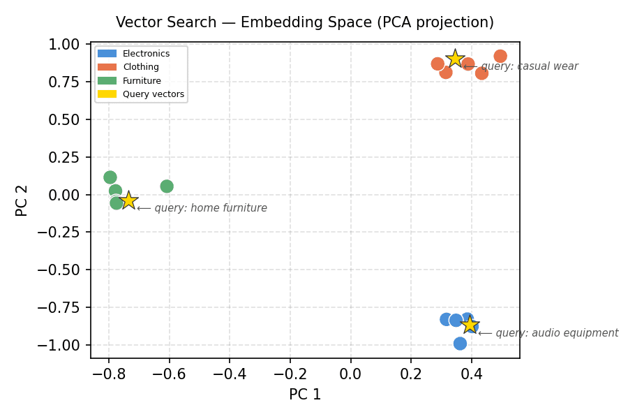
Vector Search — Embedding House (PCA projection)
The clusters separate cleanly. Every gold star (question vector) lands contained in the cluster it was constructed from. That is the geometry that vector search makes use of.
# Visualizing the Similarity Rating Distribution
For any given question, it is helpful to see how similarity scores are distributed throughout the entire index — and never simply the top-k. This tells you whether or not the highest result’s a transparent winner or simply marginally higher than every part else.
q_vec_furniture = queries["home furniture"]
q_norm_furniture = normalize(q_vec_furniture.reshape(1, -1))
all_scores_furniture = (index.vectors @ q_norm_furniture.T).flatten()

sorted_idx_furniture = np.argsort(all_scores_furniture)[::-1]
sorted_scores_furniture = all_scores_furniture[sorted_idx_furniture]
sorted_labels_furniture = [:30] + "…" if len(merchandise[i]) > 30
                           else merchandise[i] for i in sorted_idx_furniture]

# Outline bar colours: inexperienced for furnishings gadgets, grey for others
bar_colors_furniture = []
for i in sorted_idx_furniture:
    if i >= 10 and that i <= 14:  # Furnishings gadgets are initially at indices 10-14
        bar_colors_furniture.append("#5BAD72") # Inexperienced for furnishings
    else:
        bar_colors_furniture.append("#cccccc") # Grey for others

fig, ax = plt.subplots(figsize=(10, 5))
bars = ax.barh(sorted_labels_furniture[::-1], sorted_scores_furniture[::-1],
               shade=bar_colors_furniture[::-1], edgecolor="white", peak=0.65)

ax.axvline(sorted_scores_furniture[2], shade="#5BAD72", linestyle="--",
           linewidth=1.2, label="High-3 cutoff")
ax.set_xlim(sorted_scores_furniture.min() - 0.002, 1.001)
ax.set_xlabel("Cosine Similarity Rating")
ax.set_title("Question: 'dwelling furnishings' — Similarity Throughout All Merchandise", fontsize=11, pad=12)
ax.legend(fontsize=8)
ax.grid(axis="x", linestyle="--", alpha=0.4)
plt.tight_layout()
plt.savefig("score_distribution_furniture.png", dpi=150)
plt.present()
Output:
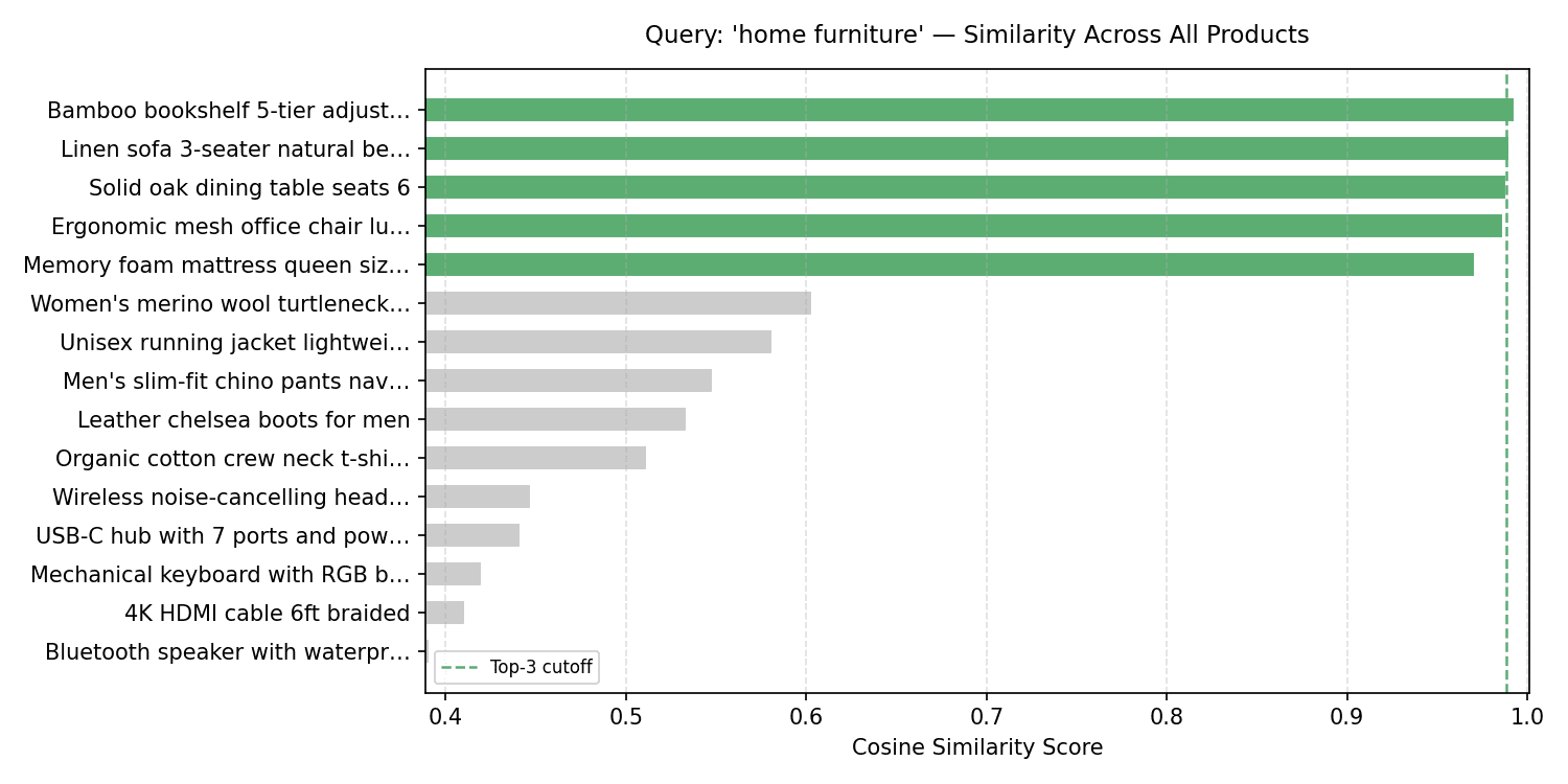
Question: ‘dwelling furnishings’ — Similarity Throughout All Merchandise
There is a seen hole between the furnishings cluster (prime 5 bars) and every part else. In observe, you’d use this hole to set a similarity threshold beneath which ends up are suppressed fully.
# Wrapping Up
You constructed a vector search engine with about 50 traces of NumPy: an index class that normalizes and shops embeddings, a search technique that makes use of matrix multiplication to compute cosine similarity, and two visualizations that reveal the geometry behind the outcomes.
The subsequent step is to switch the simulated embeddings with actual ones. Attempt loading sentence-transformers and embedding your personal textual content corpus. The index code right here will work with none adjustments.
If you would like to learn extra “from scratch” articles, tell us what you’d prefer to see subsequent!
Bala Priya C is a developer and technical author from India. She likes working on the intersection of math, programming, knowledge science, and content material creation. Her areas of curiosity and experience embody DevOps, knowledge science, and pure language processing. She enjoys studying, writing, coding, and low! At present, she’s engaged on studying and sharing her information with the developer group by authoring tutorials, how-to guides, opinion items, and extra. Bala additionally creates participating useful resource overviews and coding tutorials.


