The Geometry Behind the Dot Product: Unit Vectors, Projections, and Instinct

This text is the primary of three elements. Every half stands by itself, so that you don’t have to learn the others to know it.

The dot product is without doubt one of the most essential operations in machine studying – nevertheless it’s laborious to know with out the appropriate geometric foundations. On this first half, we construct these foundations:

· Unit vectors

· Scalar projection

· Vector projection

Whether or not you’re a scholar studying Linear Algebra for the primary time, or need to refresh these ideas, I like to recommend you learn this text.

The truth is, we’ll introduce and clarify the dot product on this article, and within the subsequent article, we’ll discover it in higher depth.

The vector projection part is included as an non-compulsory bonus: useful, however not essential for understanding the dot product.

The following half explores the dot product in higher depth: its geometric which means, its relationship to cosine similarity, and why the distinction issues.

The ultimate half connects these concepts to 2 main purposes: suggestion programs and NLP.

A vector $giant mathbf{vec{v}}$ is known as a unit vector if its magnitude is 1:

$LARGE mathbf{|vec{v}|} = 1$

To take away the magnitude of a non-zero vector whereas retaining its course, we are able to normalize it. Normalization scales the vector by the issue:

$LARGE frac{1}{|mathbf{vec{v}}|}$

The normalized vector $giant mathbf{hat{v}}$  is the unit vector within the course of $giant mathbf{vec{v}}$: 

$LARGE start{array}c hline mathbf{hat{v}} = frac{mathbf{vec{v}}}{|mathbf{vec{v}}|} hline finish{array}$

Notation 1. Any further, each time we normalize a vector $giant mathbf{vec{v}}$,  or write $giant mathbf{hat{v}}$, we assume that $giant mathbf{vec{v}} neq 0$. This notation, together with those that observe, can be related to the next articles.

This operation naturally separates a vector into its magnitude and its course:

$LARGE start{array}c hline rule{0pt}{2.5em} mathbf{vec{v}} = underbrace{|mathbf{vec{v}}|}_{textual content{magnitude}} cdot underbrace{mathbf{hat{v}}}_{textual content{course}} [4.5em] hline finish{array}$

Determine 1 illustrates this concept: ${mathbf{v}}$ and $giant mathbf{hat{v}}$ level in the identical course, however have completely different magnitudes.

Similarity of unit vectors

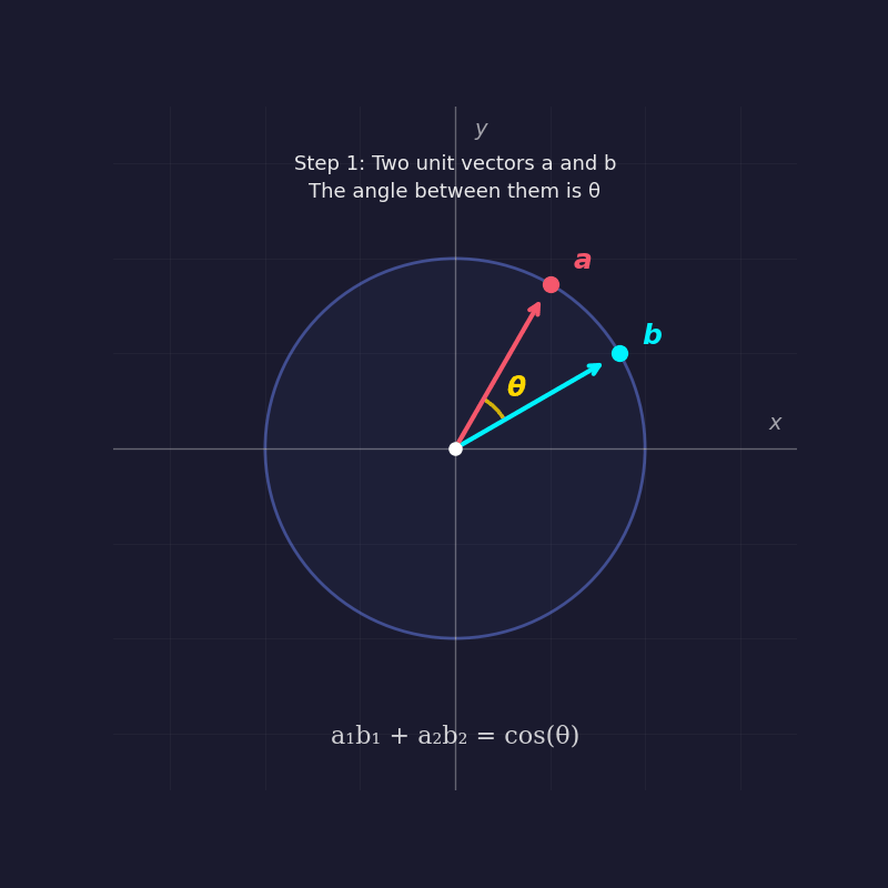
In two dimensions, all unit vectors lie on the unit circle (radius 1, centered on the origin). A unit vector that varieties an angle θ with the x-axis has coordinates (cos θ, sin θ).

This implies the angle between two unit vectors encodes a pure similarity rating - as we’ll present shortly, this rating is precisely cos θ: equal to 1 after they level the identical approach, 0 when perpendicular, and −1 when reverse.

Notation 2. All through this text, θ denotes the smallest angle between the 2 vectors, so $0° leq theta leq 180°$ .

In apply, we don’t know θ instantly – we all know the vectors’ coordinates.

We will present why the dot product of two unit vectors: $largehat{a}$ and $largehat{b}$ equals cos θ utilizing a geometrical argument in three steps:

1. Rotate the coordinate system till $largehat{b}$ lies alongside the x-axis. Rotation doesn’t change angles or magnitudes.

2. Learn off the brand new coordinates. After rotation, $largehat{b}$ has coordinates (1 , 0). Since $largehat{a}$ is a unit vector at angle θ from the x-axis, the unit circle definition provides its coordinates as (cos θ, sin θ).

3. Multiply corresponding parts and sum:

$Giant start{aligned} hat{a} cdot hat{b} = a_x cdot b_x + a_y cdot b_y = costheta cdot 1 + sintheta cdot 0 = costheta finish{aligned}$

This sum of component-wise merchandise is known as the dot product:

$Giant boxed{ start{aligned} vec{a} cdot vec{b} = a_1 cdot b_1 + a_2 cdot b_2 + cdots + a_n cdot b_n finish{aligned} }$

See the illustration of those three steps in Determine 2 beneath:

Every thing above was proven in 2D, however the identical end result holds in any variety of dimensions. Any two vectors, regardless of what number of dimensions they reside in, all the time lie in a single flat airplane. We will rotate that airplane to align with the xy-plane — and from there, the 2D proof applies precisely.

Notation 3. Within the diagrams that observe, we frequently draw one of many vectors (sometimes $largevec{b}$) alongside the horizontal axis. When $largevec{b}$ shouldn’t be already aligned with the x-axis, we are able to all the time rotate our coordinate system as we did above (the “rotation trick”). Since rotation preserves all lengths, angles, and dot merchandise, each system derived on this orientation holds for any course of $largevec{b}$.

A vector can contribute in lots of instructions directly, however usually we care about just one course.

Scalar projection solutions the query: How a lot of $giant boldsymbol{vec{a}}$ lies alongside the course of $giant boldsymbol{vec{b}}$?

This worth is damaging if the projection factors in the wrong way of $largevec{b}$.

The Shadow Analogy

Essentially the most intuitive approach to consider scalar projection is because the size of a shadow. Think about you maintain a stick (vector $giant vec{a}$) at an angle above the bottom (the course of $largevec{b}$), and a lightweight supply shines straight down from above.

The shadow that the stick casts on the bottom is the scalar projection.

The animated determine beneath illustrates this concept:

Calculation

Think about a lightweight supply shining straight down onto the road PS (the course of $largevec{b}$). The “shadow” that $largevec{a}$ (the arrow from P to Q ) casts onto that line is precisely the section PR. You may see this in Determine 4.

Deriving the system

Now have a look at the triangle $giant PQR$: the perpendicular drop from$giant Q$ creates a proper triangle, and its sides are:

• $giant PQ = |vec{a}|$ (the hypotenuse).
• $giant PR$ (the adjoining facet – the shadow).
• $giant QR$ (the other facet – the perpendicular part).

From this triangle:

1. The angle between $largevec{a}$ and $largevec{b}$ is θ.
2. $giant cos(theta) = frac{PR}{|vec{a}|}$ (probably the most primary definition of cosine).
3. Multiply each side by $giant|vec{a}|$ :

$LARGE start{array}c hline PR = |vec{a}| cos(theta) hline finish{array}$

The Phase $boldsymbol{PR}$ is the shadow size – the scalar projection of $giant boldsymbol{vec{a}}$ on $giant boldsymbol{vec{b}}$.

When θ > 90°, the scalar projection turns into damaging too. Consider the shadow as flipping to the other facet.

How is the unit vector associated?

The shadow’s size (PR) doesn’t depend upon how lengthy $largevec{b}$ is. It depends upon $giant|vec{a}|$ and on θ.

Once you compute $largevec{a} cdot hat{b}$, you might be asking: how a lot of $largevec{a}$ lies alongside $largevec{b}$ course?  That is the shadow size.

The unit vector acts like a course filter: multiplying $largevec{a}$ by it extracts the part of $largevec{a}$ alongside that course.

Let’s see it utilizing the rotation trick. We place b̂ alongside the x-axis:

$Giant vec{a} = (|vec{a}|costheta, |vec{a}|sin(theta))$

and:

$Giant hat{b} = (1, 0)$

Then:

$Giant start{aligned} vec{a} cdot hat{b} = |vec{a}|costheta cdot 1 + |vec{a}|sin(theta) cdot 0 = |vec{a}|costheta finish{aligned}$

The scalar projection of $giant boldsymbol{vec{a}}$ within the course of $giant boldsymbol{vec{b}}$ is:

$LARGE renewcommand{arraystretch}{2} start{array}c hline start{aligned} |vec{a}|costheta &= vec{a} cdot hat{b} &= frac{vec{a} cdot vec{b}}{|vec{b}|} finish{aligned} hline finish{array}$

We apply the identical rotation trick yet one more time, now with two common vectors: $largevec{a}$ and $largevec{b}$.

After rotation:

$Giant vec{a} = (|vec{a}|costheta, |vec{a}|sintheta)$ ,

$Giant vec{b} = (|vec{b}|, 0)$

so:

$Giant start{aligned} vec{a} cdot vec{b} = |vec{a}|costheta cdot |vec{b}| + |vec{a}|sintheta cdot 0 = |vec{a}||vec{b}|costheta finish{aligned}$

The dot product of $giant boldsymbol{vec{a}}$ and $giant boldsymbol{vec{b}}$ is:

$Giant renewcommand{arraystretch}{2} start{array}l hline vec{a} cdot vec{b} = a_1 b_1+ dots + a_n b_n = sum_{i=1}^{n} a_i b_i = |vec{a}||vec{b}|costheta hline finish{array}$

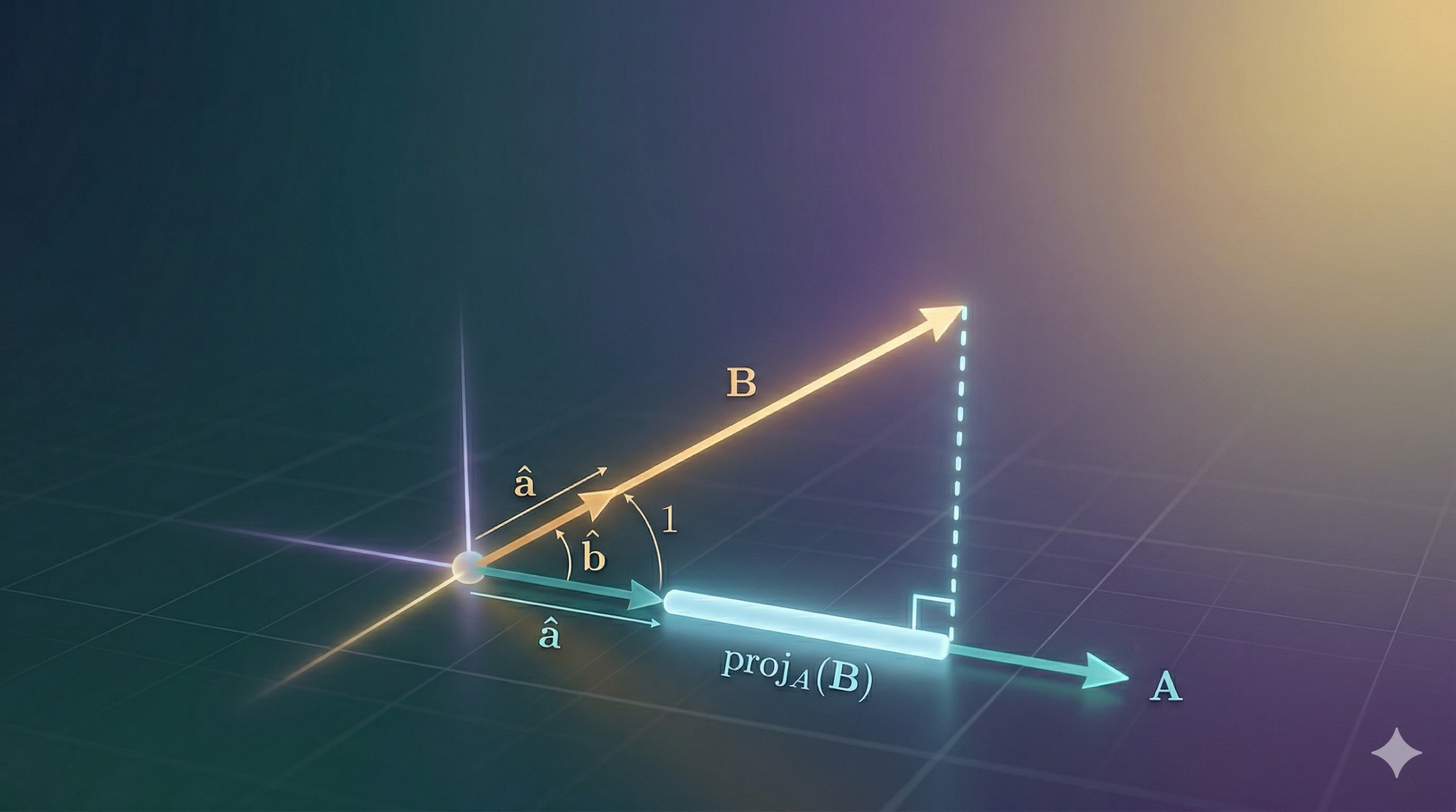
Vector projection extracts the portion of vector $giant boldsymbol{vec{a}}$ that factors alongside the course of vector $giant boldsymbol{vec{b}}$.

The Path Analogy

Think about two trails ranging from the identical level (the origin):

• Path A results in a whale-watching spot.
• Path B leads alongside the coast in a special course.

Right here’s the query projection solutions:

You’re solely allowed to stroll alongside Path B. How far do you have to stroll in order that you find yourself as shut as doable to the endpoint of Path A?

You stroll alongside B, and in some unspecified time in the future, you cease. From the place you stopped, you look towards the top of Path A, and the road connecting you to it varieties an ideal 90° angle with Path B. That’s the important thing geometric truth – the closest level is all the time the place you’d make a right-angle flip.

The spot the place you cease on Path B is the projection of A onto B. It represents “the a part of A that goes in B’s course.

The remaining hole -  out of your stopping level to the precise finish of Path A  –  is all the pieces about A that has nothing to do with B’s course. This instance is illustrated in Determine 5 beneath: The vector that begins on the origin, factors alongside Path B, and ends on the closest level –is the vector projection of $largevec{a}$ onto $largevec{b}$.

Scalar projection solutions: “How far did you stroll?”

That’s only a distance, a single quantity.

Vector projection solutions: “The place precisely are you?”

Extra exactly: “What’s the precise motion alongside Path B that will get you to that closest level?”

Now “1.5 kilometers” isn’t sufficient, you have to say “1.5 kilometers east alongside the coast.” That’s a distance plus a course: an arrow, not only a quantity. The arrow begins on the origin, factors alongside Path B, and ends on the closest level.

The space you walked is the scalar projection worth. The magnitude of the vector projection equals absolutely the worth of the scalar projection.

Unit vector  solutions : “Which course does Path B go?”

It’s precisely what $largehat{b}$ represents. It’s Path B stripped of any size info  - simply the pure course of the coast.

$start{aligned} &textual content{vector projection} = &underbrace{(textual content{how far you stroll})}_{textual content{scalar projection}} occasions underbrace{(textual content{B course})}_{hat{b}} finish{aligned}$

I do know the whale analog could be very particular; it was impressed by this good rationalization (Michael.P, 2014)

Determine 6 beneath exhibits the identical shadow diagram as in Determine 4, with PR drawn as an arrow, as a result of the vector projection is a vector (with each size and course), not only a quantity.

Because the projection should lie alongside $largevec{b}$ , we’d like two issues for $largevec{PR}$ :

1. Its magnitude is the scalar projection: $giant|vec{a}|costheta$
2. Its course is: $largehat{b}$ (the course of $largevec{b}$)

Any vector equals its magnitude occasions its course (as we noticed within the Unit Vector part), so:

$giant start{array}c hline hspace{10pt} vec{PR} = underbrace{|vec{a}| cos theta}_{textual content{scalar projection}} cdot underbrace{hat{b}}_{textual content{course of } vec{b}} hspace{20pt} hline finish{array}$

That is already the vector projection system. We will rewrite it by substituting $largehat{b} = frac{vec{b}}{|vec{b}|}$ , and recognizing that $giant|vec{a}||vec{b}|costheta = vec{a} cdot vec{b}$

The vector projection of $giant boldsymbol{vec{a}}$ within the course of $giant boldsymbol{vec{b}}$ is:

$Giant renewcommand{arraystretch}{1.5} start{array}c hline start{aligned} textual content{proj}_{vec{b}}(vec{a}) &= (|vec{a}|costheta)hat{b} &= left(frac{vec{a} cdot vec{b}}{|vec{b}|^2}proper)vec{b} &= (vec{a} cdot hat{b})hat{b} finish{aligned} hline finish{array}$

• A unit vector isolates a vector’s course by stripping away its magnitude.

$LARGE start{array}c hline mathbf{hat{v}} = frac{mathbf{vec{v}}}{|mathbf{vec{v}}|} hline finish{array}$

• The dot product multiplies corresponding parts and sums them. It’s also equal to the product of the magnitudes of the 2 vectors multiplied by the cosine of the angle between them.

$renewcommand{arraystretch}{2} start{array}l hline vec{a} cdot vec{b} = a_1 b_1+ dots + a_n b_n = sum_{i=1}^{n} a_i b_i = |vec{a}||vec{b}|costheta hline finish{array}$

• Scalar projection makes use of the dot product to measure how far one vector reaches alongside one other’s course - a single quantity, just like the size of a shadow

$Giant start{array}c hline |vec{a}|costheta = vec{a} cdot hat{b} = frac{vec{a} cdot vec{b}}{|vec{b}|} hline finish{array}$

• Vector projection goes one step additional, returning an precise arrow alongside that course: the scalar projection occasions the unit vector.

$Giant renewcommand{arraystretch}{2} start{array}l hline (|vec{a}|costheta)hat{b} = (vec{a} cdot hat{b})hat{b} hline finish{array}$

Within the subsequent half, we’ll use the instruments we discovered on this article to actually perceive the dot product.