


(CFD) is usually seen as a black field of advanced business software program. Nonetheless, implementing a solver “from scratch” is likely one of the strongest methods to study the physics of fluid movement. I began this as a private venture, and as part of a course on Biophysics, I took it as a possibility to lastly perceive how these lovely simulations work.
This information is designed for information scientists and engineers who need to transfer past high-level libraries and perceive the underlying mechanics of numerical simulations by translating partial differential equations into discretized Python code. We can even discover elementary programming ideas like vectorized operations with NumPy and stochastic convergence, that are important expertise for everybody keen on broader scientific computing and machine studying architectures.
We’ll stroll by the derivation and Python implementation of a easy incompressible Navier-Stokes (NS) solver. After which, we’ll then apply this solver to simulate airflow round a chicken’s wing profile.
The Physics: Incompressible Navier-Stokes
The basic equations of CFD are the Navier-Stokes equations, which describe how velocity and stress evolve in a fluid. For regular flight (like a chicken gliding), we assume the air is incompressible (fixed density) and laminar. They are often understood as simply Newton’s movement legislation, however for an infinitesimal aspect of fluid, with the forces that have an effect on it. That’s principally stress and viscosity, however relying on the context you could possibly add in gravity, mechanical stresses, and even electromagnetism should you’re feeling prefer it. The creator can attest to this being very a lot not advocate for a primary venture.
The equations in vector type are:
[
frac{partial mathbf{v}}{partial t} + (mathbf{v} cdot nabla)mathbf{v} = -frac{1}{rho}nabla p + nu nabla^2 mathbf{v}
nabla cdot mathbf{v} = 0
]
The place:
- v: Velocity discipline (u,v)
- p: Stress
- ρ: Fluid density
- ν: Kinematic viscosity
The primary equation (Momentum) balances inertia in opposition to stress gradients and viscous diffusion. The second equation (Continuity) enforces that the fluid density stays fixed.
The Stress Coupling Drawback
A serious problem in CFD is that stress and velocity are coupled: the stress discipline should regulate continuously to make sure the fluid stays incompressible.
To unravel this, we derive a Stress-Poisson equation by taking the divergence of the momentum equation. In a discretized solver, we remedy this Poisson equation at each single timestep to replace the stress, making certain the speed discipline stays divergence-free.
Discretization: From Math to Grid
To unravel these equations on a pc, we use Finite Distinction schemes on a uniform grid.
- Time: Ahead distinction (Specific Euler).
- Advection (Nonlinear phrases): Backward/Upwind distinction (for stability).
- Diffusion & Stress: Central distinction.
For instance, the replace formulation for the u (x-velocity) part seems to be like this in finite-difference type
[
u_{i,j}^n frac{u_{i,j}^n - u_{i-1,j}^n}{Delta x}
]
In code, the advection time period u∂x∂u makes use of a backward distinction:
[
u_{i,j}^n frac{u_{i,j}^n - u_{i-1,j}^n}{Delta x}
]
The Python Implementation
The implementation proceeds in 4 distinct steps utilizing NumPy arrays.
1. Initialization
We outline the grid dimension (nx, ny), time step (dt), and bodily parameters (rho, nu). We initialize velocity fields (u,v) and stress (p) to zeros or a uniform movement.
2. The Wing Geometry (Immersed Boundary)
To simulate a wing on a Cartesian grid, we have to mark which grid factors lie inside the strong wing.
- We load a wing mesh (e.g., from an STL file).
- We create a Boolean masks array the place
Truesignifies a degree contained in the wing. - Through the simulation, we power velocity to zero at these masked factors (no-slip/no-penetration situation).
3. The Primary Solver Loop
The core loop repeats till the answer reaches a gradual state. The steps are:
- Construct the Supply Time period (b): Calculate the divergence of the speed phrases.
- Resolve Stress: Resolve the Poisson equation for p utilizing Jacobi iteration.
- Replace Velocity: Use the brand new stress to replace u and v.
- Apply Boundary Circumstances: Implement inlet velocity and nil velocities contained in the wing.
The Code
Right here is how the core mathematical updates look in Python (vectorized for efficiency).
Step A: Constructing the Stress Supply Time period This represents the Proper-Hand Facet (RHS) of the Poisson equation primarily based on present velocities.
# b is the supply time period
# u and v are present velocity arrays
b[1:-1, 1:-1] = (rho * (
    1 / dt * ((u[1:-1, 2:] - u[1:-1, 0:-2]) / (2 * dx) +
              (v[2:, 1:-1] - v[0:-2, 1:-1]) / (2 * dy)) -
    ((u[1:-1, 2:] - u[1:-1, 0:-2]) / (2 * dx))**2 -
    2 * ((u[2:, 1:-1] - u[0:-2, 1:-1]) / (2 * dy) *
         (v[1:-1, 2:] - v[1:-1, 0:-2]) / (2 * dx)) -
    ((v[2:, 1:-1] - v[0:-2, 1:-1]) / (2 * dy))**2
))
Step B: Fixing for Stress (Jacobi Iteration) We iterate to clean out the stress discipline till it balances the supply time period.
for _ in vary(nit):
    pn = p.copy()
    p[1:-1, 1:-1] = (
        (pn[1:-1, 2:] + pn[1:-1, 0:-2]) * dy**2 +
        (pn[2:, 1:-1] + pn[0:-2, 1:-1]) * dx**2 -
        b[1:-1, 1:-1] * dx**2 * dy**2
    ) / (2 * (dx**2 + dy**2))
# Boundary situations: p=0 at edges (gauge stress)
    p[:, -1] = 0; p[:, 0] = 0; p[-1, :] = 0; p[0, :] = 0
Step C: Updating Velocity Lastly, we replace the speed utilizing the express discretized momentum equations.
un = u.copy()
vn = v.copy()
# Replace u (x-velocity)
u[1:-1, 1:-1] = (un[1:-1, 1:-1] -
                 un[1:-1, 1:-1] * dt / dx * (un[1:-1, 1:-1] - un[1:-1, 0:-2]) -
                 vn[1:-1, 1:-1] * dt / dy * (un[1:-1, 1:-1] - un[0:-2, 1:-1]) -
                 dt / (2 * rho * dx) * (p[1:-1, 2:] - p[1:-1, 0:-2]) +
                 nu * (dt / dx**2 * (un[1:-1, 2:] - 2 * un[1:-1, 1:-1] + un[1:-1, 0:-2]) +
                       dt / dy**2 * (un[2:, 1:-1] - 2 * un[1:-1, 1:-1] + un[0:-2, 1:-1])))
# Replace v (y-velocity)
v[1:-1, 1:-1] = (vn[1:-1, 1:-1] -
                 un[1:-1, 1:-1] * dt / dx * (vn[1:-1, 1:-1] - vn[1:-1, 0:-2]) -
                 vn[1:-1, 1:-1] * dt / dy * (vn[1:-1, 1:-1] - vn[0:-2, 1:-1]) -
                 dt / (2 * rho * dy) * (p[2:, 1:-1] - p[0:-2, 1:-1]) +
                 nu * (dt / dx**2 * (vn[1:-1, 2:] - 2 * vn[1:-1, 1:-1] + vn[1:-1, 0:-2]) +
                       dt / dy**2 * (vn[2:, 1:-1] - 2 * vn[1:-1, 1:-1] + vn[0:-2, 1:-1])))
Outcomes: Does it Fly?
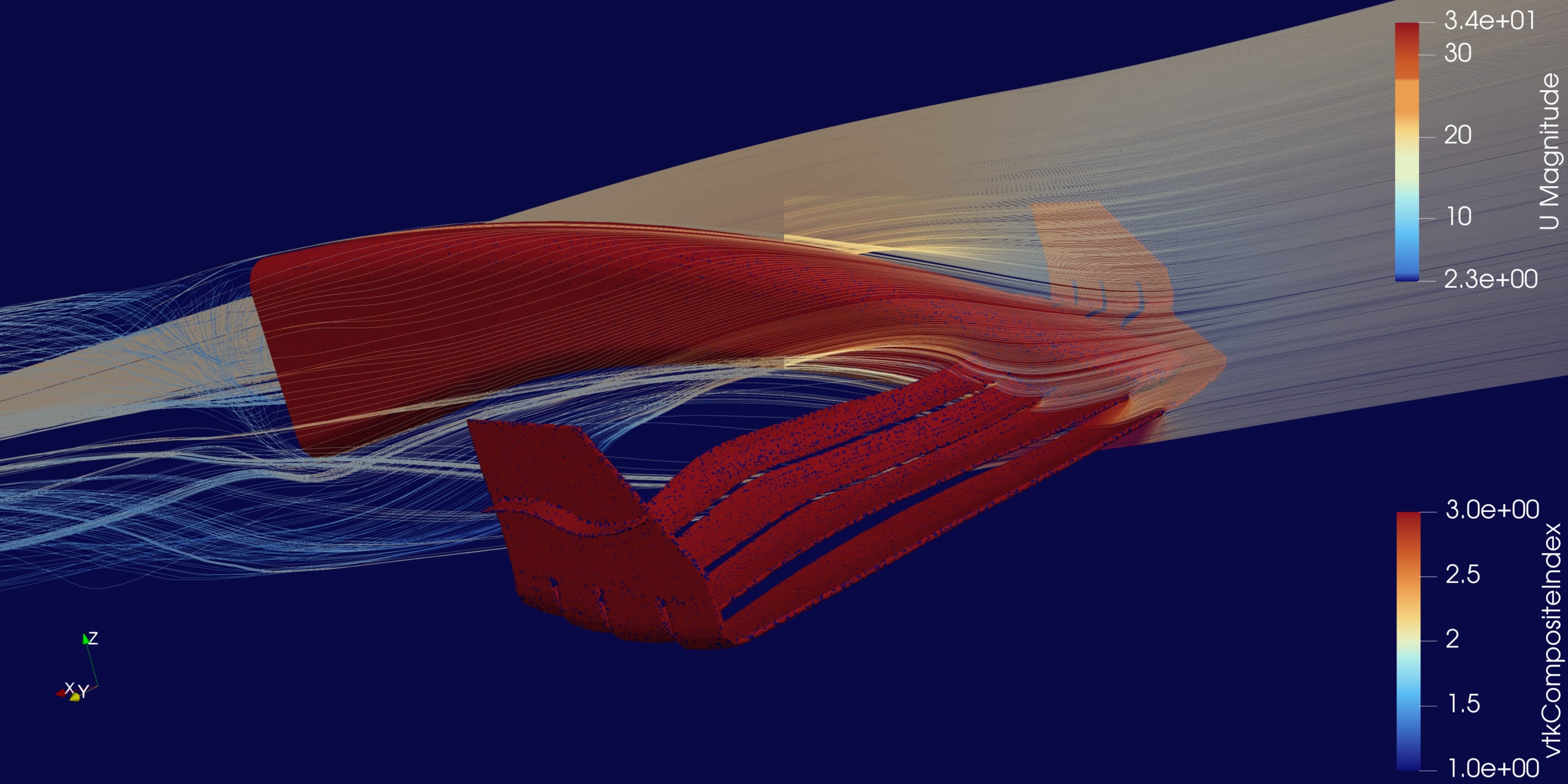
We ran this solver on a inflexible wing profile with a continuing far-field influx.

Qualitative Observations The outcomes align with bodily expectations. The simulations present excessive stress beneath the wing and low stress above it, which is strictly the mechanism that generates carry. Velocity vectors present the airflow accelerating excessive floor (Bernoulli’s precept).
Forces: Carry vs. Drag By integrating the stress discipline over the wing floor, we are able to calculate carry.
- The solver demonstrates that stress forces dominate viscous friction forces by an element of almost 1000x in air.
- Because the angle of assault will increase (from 0∘ to −20∘), the lift-to-drag ratio rises, matching traits seen in wind tunnels {and professional} CFD packages like OpenFOAM.

Limitations & Subsequent Steps
Whereas making this solver was nice for studying, the device itself has its limitations:
- Decision: 3D simulations on a Cartesian grid are computationally costly and require coarse grids, making quantitative outcomes much less dependable.
- Turbulence: The solver is laminar; it lacks a turbulence mannequin (like okay−ϵ) required for high-speed or advanced flows.
- Diffusion: Upwind differencing schemes are secure however numerically diffusive, probably “smearing” out effective movement particulars.
The place to go from right here? This venture serves as a place to begin. Future enhancements might embody implementing higher-order advection schemes (like WENO), including turbulence modeling, or shifting to Finite Quantity strategies (like OpenFOAM) for higher mesh dealing with round advanced geometries. There are many intelligent methods to get across the plethora of eventualities that you could be need to implement. That is only a first step on the path of actually understanding CFD!


