Why Random Forest Must Be This Random

“Random Forest = many timber + averaging = higher.” In the event you’ve learn even one ensemble strategies tutorial, this sentence is acquainted to the purpose of nausea. And even following probably the most primary information science tutorials, anybody will perceive that this isn’t improper. What it’s, however, is simply dangerously incomplete, as a result of if that had been the entire story, the mannequin would simply be known as “Bagged Timber,” and we’d have stopped there. We might take bootstrap samples, prepare timber, common them, achieved. No want for the phrase “Random” within the title in any respect.

However that is not what occurred. When Breiman designed Random Forest in 2001, he intentionally added a second layer of randomness: at each break up, each tree solely will get to see a random subset of the out there options; not all of them however solely a random slice.

Why? If variance had been the one downside, and bagging already reduces it by means of averaging, what does this further, seemingly restrictive constraint add? Why intentionally make your timber “extra blind”? Why cover present info out of your mannequin which may show to be important?

The reply hides in a single phrase that practitioners throw round always however hardly ever unpack mathematically: correlation. Particularly, correlation between the predictions of the timber themselves. And when you see the mathematics behind it, the entire design of Random Forest stops trying like a set of arbitrary hyperparameters and begins trying like a single, elegant argument towards a really particular enemy: correlated errors, which averaging alone can by no means totally remove, and that are precisely what stand between bagging and the algorithm’s actual potential.

That is what this text is about: why bagging alone has a tough ceiling, what is that this ceiling, and the way function subsampling is the mathematically obligatory transfer to interrupt by means of it.

Bias-Variance, a Quick Refresher

Earlier than we deep dive into the timber lets do a fast recap on how prediction error could be decomposed into three items:

Error = Bias² + Variance + Irreducible Noise

• Bias: how improper your mannequin is on common, systematically. A mannequin too easy for the underlying construction (say, a linear mannequin on nonlinear information) will constantly miss the identical means. That is underfitting.

• Variance: how a lot your mannequin’s predictions swing when you retrain it on a unique pattern from the identical distribution. A mannequin too versatile (a totally grown determination tree) will match the noise in no matter information it sees, and alter dramatically with a barely totally different coaching set. That is overfitting.

A single, unconstrained determination tree sits at one excessive of this spectrum: low bias, excessive variance. It could symbolize nearly any determination boundary (low bias), but it surely’s wildly delicate to which precise rows ended up in its coaching set (excessive variance), leading to a state of affairs the place when you swap a handful of information factors you may get a structurally totally different tree.

That is exactly why determination timber are the best uncooked materials for bagging. Bagging’s complete mechanism of averaging many fashions, is a variance-reduction instrument. It does nearly nothing for bias. So it is smart to pair it with a base learner that already has low bias and simply wants its variance tamed, somewhat than, say, bagging a bunch of linear fashions the place bias is the precise downside and averaging will not contact it.

Maintain this pairing in thoughts — bagging assaults variance, not bias — as a result of it is the idea the remainder of the article stress-tests. The query we’re about to ask is: does bagging truly ship on that promise totally, or solely partially?

The Mathematical Core: Discussing the variance computation

Suppose you may have n predictors and consider every one as a random variable $X_1, X_2, …, X_n$

Assume, for now, an idealized case:

• Every $X_i$

• The $X_i$

We will kind the ensemble prediction by averaging:

Deriving the variance of the typical

It is a direct utility of how variance propagates by means of a sum of impartial variables. For any two random variables:

If $X$ and $Y$ are impartial, Covariance can be zero and the cross-term vanishes. Generalizing to $n$ impartial variables, every scaled by $1/n$:

That is it. That is the entire derivation. No cross-terms survive as a result of independence kills each covariance time period within the enlargement.

What this says, bodily

As $nto infty$

The important thing concept behind bagging is that, below the idea of impartial timber, averaging increasingly timber repeatedly reduces the ensemble variance, finally driving it arbitrarily near zero.

The catch

As mentioned earlier than this derivation rests on one assumption that’s nearly by no means truly true in Random Forests: independence. The timber aren’t impartial. They’re skilled on bootstrap samples drawn from the identical underlying dataset, utilizing the identical options, typically discovering the identical dominant splits close to the highest of the tree. That shared construction means $Cov(X_i , X_j) neq 0$

That is precisely what the following part confronts head-on: what occurs to $Var(bar{X})$

The Twist: Timber Are By no means Really Impartial

Let’s drop the independence assumption and see what truly occurs.

Return to the uncooked definition of the variance of a sum, with out assuming independence this time:

The variance of a sum, in full generality, expands right into a double sum over all pairs $(i,j)$:

Break up this double sum into two items: the diagonal phrases the place $i=j$

When $i=j, Cov(X_i,X_i)=Var(X_i)=σ^2$

When $i neq j$

That is precisely the place the sooner derivation lower a nook: independence compelled each off-diagonal time period to zero. We not get to imagine that.

Introducing ρ

Now outline the (common) pairwise correlation between any two distinct timber:

It is a simplifying assumption — a “mean-field” therapy, precisely like assuming a uniform pairwise interplay as a substitute of monitoring each particular person pair individually. In actuality, some tree pairs are extra correlated than others (two timber that each acquired heavy weight on the identical influential outlier row, say), however treating ρ as a single common captures the combination impact cleanly, and it is a very commonplace transfer (that is primarily the identical simplification Breiman himself used within the authentic Random Forest paper).

With this substitution, the off-diagonal sum turns into:

Placing it collectively we conclude that:

and from the above level the mathematics is fairly easy to derive the ultimate expression for $Var(bar{X})$

Sanity test: setting $ρ=0$

The second time period that carries all the advantage of averaging, and contains $n$ vanishes precisely as earlier than. However the first time period $ρσ^2$, has no $n$ in it in any respect. It was by no means going to fade, irrespective of how massive $n$ will get.

The consequence

You could possibly add as many timber as you need; tens or a whole lot and even hundreds of thousands of them. Nonetheless the variance of your ensemble can by no means drop under $ρσ^2$. It is a onerous ground, set completely by how correlated your timber are, not by what number of of them you may have. Including extra timber solely ever assaults the second time period. It has zero leverage over the primary.

That is the mathematical proven fact that the complete design of Random Forest is constructed to confront. Subsequent part asks the place this $ρ$ truly comes from in an actual forest — however the analysis itself, the existence of this ground, does not depend upon any mechanism. It falls straight out of the algebra of correlated averaging, the identical means it might for correlated noise in any measurement ensemble.

Why ρ Exists, and How Random Forest Breaks It

We have proven that if timber are correlated, averaging cannot prevent as variance flooring at $ρσ^2$. So the place does that correlation truly come from?

The trigger

Each tree sees a unique bootstrap pattern, however the identical underlying dataset. If one function is a powerful predictor (say, “worth of a product”), it is going to win the best-split check on the root of practically each tree, nearly no matter which rows acquired sampled as a result of it is structurally the strongest sign within the information and never an artifact of any explicit pattern. So timber find yourself with comparable top-level construction, make comparable errors in the identical areas, and their predictions transfer collectively. Bootstrap sampling shuffles rows, but it surely does not contact which function dominates main it to decorrelate noise and never sign.

The Random Forest repair

Random Forest assaults this straight: at each single break up, every tree is barely allowed to contemplate a random subset of options (sometimes $displaystylesqrt{p}$

That’s the complete concept. Bagging randomizes the coaching rows, which reduces the variance of every particular person tree. Random Forest goes one step additional by additionally randomizing the options at each break up. This reduces the correlation $ρ$ between tree predictions, and it’s $ρ$ somewhat than the variety of timber $n$ that limits how a lot the ensemble variance could be diminished

The Experiment — What We’re Really Testing

Concept is convincing, however nothing beats seeing the numbers transfer. So we arrange a managed comparability: construct the precise situation the speculation describes, then measure $ρ, σ^2$

The setup (code on the finish of the article)

We generate an artificial inhabitants with 30 options, the place two options are intentionally made dominant (they carry a lot of the true predictive sign) whereas the remaining vary from weakly informative to pure noise. This mirrors a sensible dataset: a couple of robust drivers, a handful of secondary ones, and plenty of muddle. It is precisely the type of construction that ought to push plain bagged timber towards excessive correlation, since each tree has each incentive to separate on the identical dominant options first.

The important thing methodological alternative

That is the place the sooner dialogue about conditional vs. unconditional correlation truly issues for the experiment design, not only for the speculation. If we skilled many timber on bootstrap samples of 1 fastened coaching set, we would be measuring conditional correlation and as we labored out, that correlation is precisely zero for independently-drawn bootstrap samples, irrespective of how a lot these samples overlap in content material. That is a mathematical truth, not a subtlety we are able to sidestep.

Breiman’s $ρ$ is unconditional: it treats the coaching set itself as a random draw from the inhabitants. So to measure it actually, every impartial “trial” of our experiment has to incorporate a recent coaching set, drawn anew from the inhabitants, not simply recent bootstrap indices from the identical fastened set. All of the timber inside one trial share that one training-set draw — and that shared draw is the precise, actual supply of correlation between them.

What we do, step-by-step

1. Run many impartial trials (400 in our case). In every trial: draw a brand-new coaching set from the inhabitants, then prepare a big batch of timber on bootstrap resamples of it.

2. Do that twice; as soon as the place each tree considers all 30 options at each break up (plain bagging), and as soon as the place each tree solely considers a random subset of options at each break up (Random Forest, roughly $sqrt{30} ≈ 5–6$

3. At a set set of check factors, document each tree’s prediction, in each trial.

What we measure from that information

• ρ: how equally two totally different timber behave, on the identical check level, throughout impartial trials. Principally, if we reran the entire experiment, would tree A and tree B have a tendency to maneuver collectively?

• σ²: how a lot a single tree’s prediction, at a set check level, varies throughout impartial trials.

• Var(imply) vs. n: for a rising variety of timber n, how a lot does the ensemble’s averaged prediction fluctuate throughout impartial trials?

If the speculation holds, the third amount ought to hint out precisely $ρσ^2 + (1-ρ)σ^2/n$

The Outcomes

Here is what got here out of working the experiment described above (400 impartial trials, as much as 120 timber per ensemble):

Correlation and individual-tree variance

Two issues leap out instantly.

First, ρ drops by roughly 3.2x as soon as function subsampling is launched (0.136 → 0.043). Hiding the dominant options from most splits genuinely breaks the shared construction between timber. Somewhat than repeatedly constructing practically equivalent timber across the identical few informative variables, Random Forest encourages numerous tree constructions. This range reduces the tendency of timber to make the identical prediction errors, resulting in a a lot decrease inter-tree correlation.

Second, and fewer apparent: Random Forest’s particular person timber are literally worse. σ² is roughly double for RF (17.42 vs 9.89); a single Random Forest tree, by itself, is a noisier predictor than a single bagged tree. This is smart: proscribing every break up to ~5–6 out of 30 options typically forces the tree away from the very best out there break up, making that one tree extra erratic. Characteristic subsampling is not a free lunch on the degree of a single tree — it is a commerce: particular person high quality for diminished correlation.

Third and extra importantly, the asymptotic variance ground $ρσ^2$ decreases from 1.34 to 0.76. This demonstrates the important thing precept behind Random Forest: bettering ensemble efficiency doesn’t require stronger particular person timber, however somewhat a set of sufficiently correct timber whose prediction errors are much less correlated. Consequently, including extra timber yields a decrease limiting ensemble variance than plain bagging.

Ensemble variance vs. variety of timber

Two patterns price sitting with:

• The speculation column and the empirical column monitor one another carefully, all over.
  This is not assured — the method $Var(bar{X}) = ρσ^2 +displaystyle frac{(1-ρ)σ^2}{n}$

• The crossover
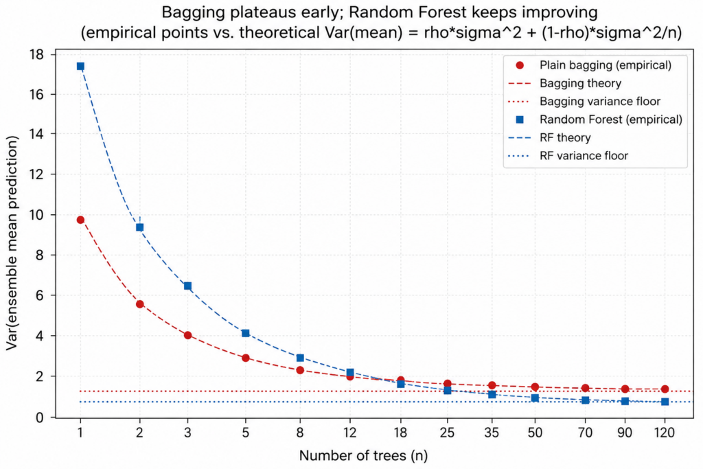
  At n=1, Random Forest begins behind as its lone tree is sort of twice as noisy as bagging’s lone tree (17.42 vs 9.89). However by round n=18, RF has already caught up and overtaken bagging (1.68 vs 1.85). By n=120, RF is sitting at roughly 59% of bagging’s variance (0.85 vs 1.44), regardless of ranging from individually worse constructing blocks.

That crossover is the complete article compressed into one sentence. Averaging alone cannot rescue plain bagging — irrespective of what number of bagged timber you add, you are caught above $ρσ² ≈$

All of the above could be compressed within the following illustrated picture generated by the code within the appendix.

The Delicate Level: Worse Timber, Higher Forest

It is price pausing on one thing that earlier sections numbers already confirmed, as a result of it is the element that surprises individuals who have used Random Forest for years with out digging into why it really works: a single Random Forest tree is a strictly worse predictor than a single bagged tree, and but the Random Forest ensemble finally ends up strictly higher.

This is not a contradiction however the complete level, when you separate two issues which might be simple to conflate:

• Particular person high quality (how good is one tree, by itself): bagging wins right here. σ² = 9.89 for bagging vs 17.42 for RF. Clearly, a bagged tree, seeing all 30 options at each break up, merely makes higher particular person selections.

• Ensemble high quality (how good is the common of many timber): RF wins right here, and never narrowly as at n=120, RF’s ensemble variance is 0.85 vs bagging’s 1.44, roughly 41% decrease.

The mechanism connecting these is completely about $ρ$, not $σ^2$. Characteristic subsampling does not make timber higher — if something, it makes every one a bit worse, because it’s sometimes compelled away from the strongest out there break up. What it buys is independence between the errors totally different timber make. And since the ensemble variance method weights $ρ$ so closely (recall: $ρ$ survives untouched as $nto infty$

It is a genuinely counter-intuitive commerce for anybody used to considering “higher base learner → higher ensemble.” For Random Forest particularly, the alternative can maintain: a barely worse base learner, if it is much less correlated with its friends, produces a meaningfully higher ensemble. It is the identical logic behind why a portfolio of mediocre, uncorrelated bets can outperform a portfolio of wonderful, extremely correlated ones; diversification has actual worth, and it might outweigh particular person high quality when you’re combining many issues.

Sensible Takeaway: max_features Is not a Element

If there’s one parameter in sklearn.ensemble.RandomForestRegressor (or RandomForestClassifier) that will get set as soon as to 'sqrt' and by no means touched once more, it is max_features. The outcomes above recommend that is typically leaving one thing on the desk.

The tradeoff, made concrete

max_features controls precisely the amount this complete article has been about: what number of options every break up can see, which straight trades off $σ²$ towards $ρ$.

• Too excessive (near, or equal to, all options — i.e. plain bagging): each tree gravitates towards the identical dominant options, and also you hit the ground early. Including extra timber previous that time burns compute for primarily nothing.

• Too low (e.g. 1 function per break up): timber change into so restricted they’re barely higher than random guessing at every break up, and the ground, whereas decrease in $ρ$ phrases, can find yourself larger in absolute Var(imply) phrases as a result of $σ²$ has grown quicker than $ρ$ shrank.

Someplace between these two extremes is a candy spot — and the place it sits depends upon the information, particularly on what number of options are genuinely dominant versus what number of carry actual, if secondary, sign.

The one-line psychological mannequin to hold ahead

max_features is not a randomness dial you set and neglect — it is the lever that decides the place your forest sits on the $σ² – ρ$

Appendix

Right here you’ll find the code I constructed and used for the evaluation. Be at liberty to execute and reproduce my outcomes or experiment with totally different parameters. (Estimated time of run ~ 7 minutes)

"""Bagging vs Random Forest: measuring rho (tree correlation) and thevariance ground Var(imply) = rho*sigma^2 + (1-rho)*sigma^2/n.KEY METHODOLOGICAL POINT:With a FIXED coaching set, if every tree's bootstrap pattern is drawnindependently, tree predictions are mathematically INDEPENDENT (rho = 0precisely) -- this follows from a primary chance truth: if A and B areimpartial random variables, then g(A) and h(B) are impartial for anyfeatures g, h, even g = h. This holds irrespective of how nonlinear ordiscontinuous the tree-fitting perform is, and althoughany two bootstrap samples will sometimes overlap closely in content material --overlap in realized values doesn't indicate statistical dependence.The correlation rho in Breiman's method is UNCONDITIONAL: it requiresthe coaching set itself to be random (drawn from the inhabitants) throughoutrepeats. All timber in a repeat share that one training-set draw, which isthe precise frequent supply of dependence. So every impartial "repeat" ofthis experiment should redraw the coaching set recent, not simply thebootstrap indices."""import numpy as npfrom sklearn.tree import DecisionTreeRegressorimport matplotlib.pyplot as pltimport timeRNG_GLOBAL = np.random.default_rng(0)# -----------------------------------------------------------------# Knowledge-generating course of: a few DOMINANT options, a number of# weaker informative options, and pure noise options.# -----------------------------------------------------------------N_TRAIN = 400N_FEATURES = 30TRUE_COEF = np.zeros(N_FEATURES)TRUE_COEF[0] = 4.0TRUE_COEF[1] = 2.5TRUE_COEF[2:8] = 0.5NOISE_SCALE = 1.5X_PROBE = RNG_GLOBAL.regular(measurement=(25, N_FEATURES))  # fastened analysis factorsdef run_repeats(max_features, R, n_max, seed0, max_depth=5):    """R impartial repeats. Every repeat: draw a FRESH coaching set from    the inhabitants, then prepare n_max timber on bootstrap resamples of it    (with the given max_features coverage). Returns predictions on the    fastened probe factors, form (R, n_max, n_probe).    """    preds = np.empty((R, n_max, X_PROBE.form[0]))    for r in vary(R):        rng = np.random.default_rng(seed0 + r)        X_train = rng.regular(measurement=(N_TRAIN, N_FEATURES))        y_train = X_train @ TRUE_COEF + rng.regular(scale=NOISE_SCALE, measurement=N_TRAIN)        for t in vary(n_max):            idx = rng.integers(0, N_TRAIN, measurement=N_TRAIN)  # bootstrap rows            Xb, yb = X_train[idx], y_train[idx]            tree = DecisionTreeRegressor(                max_features=max_features,   # None = bagging, 'sqrt' = RF                max_depth=max_depth,                random_state=rng.integers(0, 1_000_000),            )            tree.match(Xb, yb)            preds[r, t, :] = tree.predict(X_PROBE)    return predsdef pairwise_rho(preds, n_slots=10):    """Common pairwise correlation between distinct tree 'slots', throughout    impartial repeats, at fastened check factors (unconditional rho, per    Breiman's definition).    """    slots = preds[:, :n_slots, :]    rhos = []    for ok in vary(slots.form[2]):        mat = slots[:, :, k]        corr = np.corrcoef(mat, rowvar=False)        off = corr.sum() - np.hint(corr)        n_pairs = n_slots * (n_slots - 1)        rhos.append(off / n_pairs)    return float(np.nanmean(rhos))def individual_tree_variance(preds):    return float(preds[:, 0, :].var(axis=0).imply())def empirical_var_of_mean(preds, n_values):    out = []    for n in n_values:        cum_mean = preds[:, :n, :].imply(axis=1)   # (R, n_probe)        var_per_point = cum_mean.var(axis=0)        out.append(float(var_per_point.imply()))    return np.array(out)# -----------------------------------------------------------------# Run the experiment# -----------------------------------------------------------------R = 400            # impartial repeats (cut back to ~100 for a quicker run)N_MAX = 120         # max ensemble measurement probedN_VALUES = np.array([1, 2, 3, 5, 8, 12, 18, 25, 35, 50, 70, 90, 120])t0 = time.time()preds_bag = run_repeats(max_features=None, R=R, n_max=N_MAX, seed0=10_000)t1 = time.time()print(f"Bagging: {t1-t0:.1f}s")preds_rf = run_repeats(max_features="sqrt", R=R, n_max=N_MAX, seed0=50_000)t2 = time.time()print(f"RF: {t2-t1:.1f}s")rho_bag = pairwise_rho(preds_bag)rho_rf = pairwise_rho(preds_rf)sigma2_bag = individual_tree_variance(preds_bag)sigma2_rf = individual_tree_variance(preds_rf)floor_bag = rho_bag * sigma2_bagfloor_rf = rho_rf * sigma2_rfvar_bag = empirical_var_of_mean(preds_bag, N_VALUES)var_rf = empirical_var_of_mean(preds_rf, N_VALUES)print(f"nrho:        bagging={rho_bag:.4f}   RF={rho_rf:.4f}")print(f"sigma^2:    bagging={sigma2_bag:.3f}   RF={sigma2_rf:.3f}")print(f"ground:      bagging={floor_bag:.3f}   RF={floor_rf:.3f}")print(f"n{'n':>5} {'bag_emp':>10} {'bag_theory':>11} {'rf_emp':>10} {'rf_theory':>11}")for n, vb, vr in zip(N_VALUES, var_bag, var_rf):    tb = rho_bag * sigma2_bag + (1 - rho_bag) * sigma2_bag / n    tr = rho_rf * sigma2_rf + (1 - rho_rf) * sigma2_rf / n    print(f"{n:>5} {vb:>10.3f} {tb:>11.3f} {vr:>10.3f} {tr:>11.3f}")# -----------------------------------------------------------------# Plot# -----------------------------------------------------------------fig, ax = plt.subplots(figsize=(9, 6))n_smooth = np.linspace(1, N_VALUES.max(), 300)theory_bag = rho_bag*sigma2_bag + (1-rho_bag)*sigma2_bag/n_smooththeory_rf = rho_rf*sigma2_rf + (1-rho_rf)*sigma2_rf/n_smoothax.plot(N_VALUES, var_bag, "o", coloration="#d62728", label="Plain bagging (empirical)", markersize=6, zorder=5)ax.plot(n_smooth, theory_bag, "--", coloration="#d62728", alpha=0.6, label=f"Bagging principle (rho={rho_bag:.3f})")ax.axhline(floor_bag, coloration="#d62728", linestyle=":", alpha=0.5, linewidth=1.5)ax.plot(N_VALUES, var_rf, "s", coloration="#1f77b4", label="Random Forest (empirical)", markersize=6, zorder=5)ax.plot(n_smooth, theory_rf, "--", coloration="#1f77b4", alpha=0.6, label=f"RF principle (rho={rho_rf:.3f})")ax.axhline(floor_rf, coloration="#1f77b4", linestyle=":", alpha=0.5, linewidth=1.5)ax.textual content(N_VALUES.max()*0.65, floor_bag+0.05, f"bagging ground = rho*sigma^2 = {floor_bag:.2f}", coloration="#d62728", fontsize=9)ax.textual content(N_VALUES.max()*0.65, floor_rf+0.05, f"RF ground = rho*sigma^2 = {floor_rf:.2f}", coloration="#1f77b4", fontsize=9)ax.set_xlabel("Variety of timber (n)", fontsize=12)ax.set_ylabel("Var(ensemble imply prediction)", fontsize=12)ax.set_title("Bagging plateaus early; Random Forest retains improvingn"              "(empirical factors vs. theoretical Var(imply) = rho*sigma^2 + (1-rho)*sigma^2/n)", fontsize=12)ax.legend(fontsize=9, loc="higher proper")ax.set_ylim(backside=0)ax.grid(alpha=0.3)plt.tight_layout()plt.present()

References:

Breiman, L. (2001). Random Forests. Machine Studying, 45(1), 5–32.