


bushes are a preferred supervised studying algorithm with advantages that embody having the ability to be used for each regression and classification in addition to being simple to interpret. Nevertheless, determination bushes aren’t probably the most performant algorithm and are vulnerable to overfitting attributable to small variations within the coaching information. This can lead to a very totally different tree. That is why individuals typically flip to ensemble fashions like Bagged Bushes and Random Forests. These include a number of determination bushes skilled on bootstrapped information and aggregated to realize higher predictive efficiency than any single tree may provide. This tutorial contains the next:
- What’s Bagging
- What Makes Random Forests Totally different
- Coaching and Tuning a Random Forest utilizing Scikit-Be taught
- Calculating and Deciphering Function Significance
- Visualizing Particular person Choice Bushes in a Random Forest
As all the time, the code used on this tutorial is obtainable on my GitHub. A video model of this tutorial can be obtainable on my YouTube channel for many who desire to comply with alongside visually. With that, let’s get began!
What’s Bagging (Bootstrap Aggregating)

Random forests could be categorized as bagging algorithms (bootstrap aggregating). Bagging consists of two steps:
1.) Bootstrap sampling: Create a number of coaching units by randomly drawing samples with substitute from the unique dataset. These new coaching units, known as bootstrapped datasets, sometimes include the identical variety of rows as the unique dataset, however particular person rows might seem a number of instances or in no way. On common, every bootstrapped dataset incorporates about 63.2% of the distinctive rows from the unique information. The remaining ~36.8% of rows are unnoticed and can be utilized for out-of-bag (OOB) analysis. For extra on this idea, see my sampling with and with out substitute weblog publish.
2.) Aggregating predictions: Every bootstrapped dataset is used to coach a unique determination tree mannequin. The ultimate prediction is made by combining the outputs of all particular person bushes. For classification, that is sometimes accomplished by majority voting. For regression, predictions are averaged.
Coaching every tree on a unique bootstrapped pattern introduces variation throughout bushes. Whereas this doesn’t absolutely remove correlation—particularly when sure options dominate—it helps scale back overfitting when mixed with aggregation. Averaging the predictions of many such bushes reduces the general variance of the ensemble, bettering generalization.
What Makes Random Forests Totally different

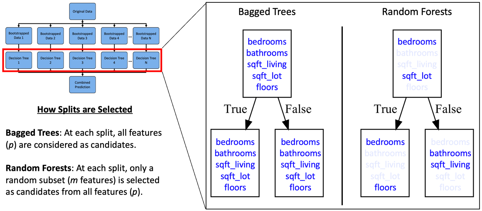
Suppose there’s a single robust function in your dataset. In bagged bushes, every tree might repeatedly break up on that function, resulting in correlated bushes and fewer profit from aggregation. Random Forests scale back this problem by introducing additional randomness. Particularly, they modify how splits are chosen throughout coaching:
1). Create N bootstrapped datasets. Word that whereas bootstrapping is usually utilized in Random Forests, it isn’t strictly mandatory as a result of step 2 (random function choice) introduces adequate variety among the many bushes.
2). For every tree, at every node, a random subset of options is chosen as candidates, and the most effective break up is chosen from that subset. In scikit-learn, that is managed by the max_features parameter, which defaults to 'sqrt' for classifiers and 1 for regressors (equal to bagged bushes).
3). Aggregating predictions: vote for classification and common for regression.
Word: Random Forests use sampling with substitute for bootstrapped datasets and sampling with out substitute for choosing a subset of options.

Out-of-Bag (OOB) Rating
As a result of ~36.8% of coaching information is excluded from any given tree, you should utilize this holdout portion to judge that tree’s predictions. Scikit-learn permits this through the oob_score=True parameter, offering an environment friendly option to estimate generalization error. You’ll see this parameter used within the coaching instance later within the tutorial.
Coaching and Tuning a Random Forest in Scikit-Be taught
Random Forests stay a powerful baseline for tabular information because of their simplicity, interpretability, and skill to parallelize since every tree is skilled independently. This part demonstrates the best way to load information, carry out a prepare take a look at break up, prepare a baseline mannequin, tune hyperparameters utilizing grid search, and consider the ultimate mannequin on the take a look at set.
Step 1: Prepare a Baseline Mannequin
Earlier than tuning, it’s good follow to coach a baseline mannequin utilizing cheap defaults. This offers you an preliminary sense of efficiency and allows you to validate generalization utilizing the out-of-bag (OOB) rating, which is constructed into bagging-based fashions like Random Forests. This instance makes use of the Home Gross sales in King County dataset (CCO 1.0 Common License), which incorporates property gross sales from the Seattle space between Could 2014 and Could 2015. This method permits us to order the take a look at set for ultimate analysis after tuning.
Python"># Import libraries

# Some imports are solely used later within the tutorial
import matplotlib.pyplot as plt

import numpy as np

import pandas as pd

# Dataset: Breast Most cancers Wisconsin (Diagnostic)
# Supply: UCI Machine Studying Repository
# License: CC BY 4.0
from sklearn.datasets import load_breast_cancer

from sklearn.ensemble import RandomForestClassifier

from sklearn.ensemble import RandomForestRegressor

from sklearn.inspection import permutation_importance

from sklearn.model_selection import GridSearchCV, train_test_split

from sklearn import tree

# Load dataset
# Dataset: Home Gross sales in King County (Could 2014–Could 2015)
# License CC0 1.0 Common
url = 'https://uncooked.githubusercontent.com/mGalarnyk/Tutorial_Data/grasp/King_County/kingCountyHouseData.csv'

df = pd.read_csv(url)

columns = ['bedrooms',

            'bathrooms',

            'sqft_living',

            'sqft_lot',

             'floors',

             'waterfront',

             'view',

             'condition',

             'grade',

             'sqft_above',

             'sqft_basement',

             'yr_built',

             'yr_renovated',

             'lat',

             'long',

             'sqft_living15',

             'sqft_lot15',

             'price']

df = df[columns]

# Outline options and goal

X = df.drop(columns='value')

y = df['price']

# Prepare/take a look at break up

X_train, X_test, y_train, y_test = train_test_split(X, y, random_state=0)

# Prepare baseline Random Forest

reg = RandomForestRegressor(

    n_estimators=100,        # variety of bushes

    max_features=1/3,        # fraction of options thought-about at every break up

    oob_score=True,          # permits out-of-bag analysis

    random_state=0

)

reg.match(X_train, y_train)

# Consider baseline efficiency utilizing OOB rating

print(f"Baseline OOB rating: {reg.oob_score_:.3f}")
Step 2: Tune Hyperparameters with Grid Search
Whereas the baseline mannequin provides a powerful place to begin, efficiency can typically be improved by tuning key hyperparameters. Grid search cross-validation, as applied by GridSearchCV, systematically explores mixtures of hyperparameters and makes use of cross-validation to judge each, choosing the configuration with the very best validation efficiency.Probably the most generally tuned hyperparameters embody:
n_estimators: The variety of determination bushes within the forest. Extra bushes can enhance accuracy however enhance coaching time.max_features: The variety of options to contemplate when on the lookout for the most effective break up. Decrease values scale back correlation between bushes.max_depth: The utmost depth of every tree. Shallower bushes are quicker however might underfit.min_samples_split: The minimal variety of samples required to separate an inner node. Larger values can scale back overfitting.min_samples_leaf: The minimal variety of samples required to be at a leaf node. Helps management tree dimension.bootstrap: Whether or not bootstrap samples are used when constructing bushes. If False, the entire dataset is used.
param_grid = {

    'n_estimators': [100],

    'max_features': ['sqrt', 'log2', None],

    'max_depth': [None, 5, 10, 20],

    'min_samples_split': [2, 5],

    'min_samples_leaf': [1, 2]

}

# Initialize mannequin

rf = RandomForestRegressor(random_state=0, oob_score=True)

grid_search = GridSearchCV(

    estimator=rf,

    param_grid=param_grid,

    cv=5,             # 5-fold cross-validation

    scoring='r2',     # analysis metric

    n_jobs=-1         # use all obtainable CPU cores

)

grid_search.match(X_train, y_train)

print(f"Finest parameters: {grid_search.best_params_}")

print(f"Finest R^2 rating: {grid_search.best_score_:.3f}")
Step 3: Consider Remaining Mannequin on Check Set
Now that we’ve chosen the best-performing mannequin based mostly on cross-validation, we are able to consider it on the held-out take a look at set to estimate its generalization efficiency.
# Consider ultimate mannequin on take a look at set

best_model = grid_search.best_estimator_

print(f"Check R^2 rating (ultimate mannequin): {best_model.rating(X_test, y_test):.3f}")
Calculating Random Forest Function Significance
One of many key benefits of Random Forests is their interpretability — one thing that enormous language fashions (LLMs) typically lack. Whereas LLMs are highly effective, they sometimes perform as black containers and might exhibit biases which are tough to determine. In distinction, scikit-learn helps two essential strategies for measuring function significance in Random Forests: Imply Lower in Impurity and Permutation Significance.
1). Imply Lower in Impurity (MDI): Often known as Gini significance, this methodology calculates the full discount in impurity introduced by every function throughout all bushes. That is quick and constructed into the mannequin through reg.feature_importances_. Nevertheless, impurity-based function importances could be deceptive, particularly for options with excessive cardinality (many distinctive values), as these options usually tend to be chosen just because they supply extra potential break up factors.
importances = reg.feature_importances_

feature_names = X.columns

sorted_idx = np.argsort(importances)[::-1]

for i in sorted_idx:

    print(f"{feature_names[i]}: {importances[i]:.3f}")
2). Permutation Significance: This methodology assesses the lower in mannequin efficiency when a single function’s values are randomly shuffled. In contrast to MDI, it accounts for function interactions and correlation. It’s extra dependable but in addition extra computationally costly.
# Carry out permutation significance on the take a look at set

perm_importance = permutation_importance(reg, X_test, y_test, n_repeats=10, random_state=0)

sorted_idx = perm_importance.importances_mean.argsort()[::-1]

for i in sorted_idx:

    print(f"{X.columns[i]}: {perm_importance.importances_mean[i]:.3f}")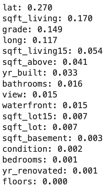
It is very important be aware that our geographic options lat and lengthy are additionally helpful for visualization because the plot beneath exhibits. It’s probably that corporations like Zillow leverage location info extensively of their valuation fashions.

Visualizing Particular person Choice Bushes in a Random Forest
A Random Forest consists of a number of determination bushes—one for every estimator specified through the n_estimators parameter. After coaching the mannequin, you may entry these particular person bushes by the .estimators_ attribute. Visualizing a number of of those bushes may also help illustrate how in another way each splits the information attributable to bootstrapped coaching samples and random function choice at every break up. Whereas the sooner instance used a RandomForestRegressor, right here we reveal this visualization utilizing a RandomForestClassifier skilled on the Breast Most cancers Wisconsin dataset (CC BY 4.0 license) to spotlight Random Forests’ versatility for each regression and classification duties. This quick video demonstrates what 100 skilled estimators from this dataset appear to be.
Match a Random Forest Mannequin utilizing Scikit-Be taught
# Load the Breast Most cancers (Diagnostic) Dataset

information = load_breast_cancer()

df = pd.DataFrame(information.information, columns=information.feature_names)

df['target'] = information.goal

# Organize Information into Options Matrix and Goal Vector

X = df.loc[:, df.columns != 'target']

y = df.loc[:, 'target'].values

# Cut up the information into coaching and testing units

X_train, X_test, Y_train, Y_test = train_test_split(X, y, random_state=0)

# Random Forests in `scikit-learn` (with N = 100)

rf = RandomForestClassifier(n_estimators=100,

                            random_state=0)

rf.match(X_train, Y_train)
Plotting Particular person Estimators (determination bushes) from a Random Forest utilizing Matplotlib
Now you can view all the person bushes from the fitted mannequin.
rf.estimators_

Now you can visualize particular person bushes. The code beneath visualizes the primary determination tree.
fn=information.feature_names

cn=information.target_names

fig, axes = plt.subplots(nrows = 1,ncols = 1,figsize = (4,4), dpi=800)

tree.plot_tree(rf.estimators_[0],

               feature_names = fn,

               class_names=cn,

               crammed = True);

fig.savefig('rf_individualtree.png')
Though plotting many bushes could be tough to interpret, you could want to discover the variability throughout estimators. The next instance exhibits the best way to visualize the primary 5 determination bushes within the forest:
# This will likely not the easiest way to view every estimator as it's small

fig, axes = plt.subplots(nrows=1, ncols=5, figsize=(10, 2), dpi=3000)

for index in vary(5):

    tree.plot_tree(rf.estimators_[index],

                   feature_names=fn,

                   class_names=cn,

                   crammed=True,

                   ax=axes[index])

    axes[index].set_title(f'Estimator: {index}', fontsize=11)

fig.savefig('rf_5trees.png')
Conclusion
Random forests include a number of determination bushes skilled on bootstrapped information so as to obtain higher predictive efficiency than could possibly be obtained from any of the person determination bushes. When you’ve got questions or ideas on the tutorial, be happy to achieve out by YouTube or X.


