


AutoBNN combines the interpretability of conventional probabilistic approaches with the scalability and adaptability of neural networks for constructing refined time sequence prediction fashions utilizing complicated information.
Time sequence issues are ubiquitous, from forecasting climate and site visitors patterns to understanding financial developments. Bayesian approaches begin with an assumption concerning the information’s patterns (prior likelihood), accumulating proof (e.g., new time sequence information), and repeatedly updating that assumption to type a posterior likelihood distribution. Conventional Bayesian approaches like Gaussian processes (GPs) and Structural Time Collection are extensively used for modeling time sequence information, e.g., the generally used Mauna Loa CO2 dataset. Nevertheless, they usually depend on area consultants to painstakingly choose applicable mannequin elements and could also be computationally costly. Options similar to neural networks lack interpretability, making it obscure how they generate forecasts, and do not produce dependable confidence intervals.
To that finish, we introduce AutoBNN, a brand new open-source bundle written in JAX. AutoBNN automates the invention of interpretable time sequence forecasting fashions, gives high-quality uncertainty estimates, and scales successfully to be used on giant datasets. We describe how AutoBNN combines the interpretability of conventional probabilistic approaches with the scalability and adaptability of neural networks.
AutoBNN
AutoBNN relies on a line of analysis that over the previous decade has yielded improved predictive accuracy by modeling time sequence utilizing GPs with discovered kernel constructions. The kernel operate of a GP encodes assumptions concerning the operate being modeled, such because the presence of developments, periodicity or noise. With discovered GP kernels, the kernel operate is outlined compositionally: it’s both a base kernel (similar to Linear, Quadratic, Periodic, Matérn or ExponentiatedQuadratic) or a composite that mixes two or extra kernel features utilizing operators similar to Addition, Multiplication, or ChangePoint. This compositional kernel construction serves two associated functions. First, it’s easy sufficient {that a} consumer who’s an professional about their information, however not essentially about GPs, can assemble an inexpensive prior for his or her time sequence. Second, strategies like Sequential Monte Carlo can be utilized for discrete searches over small constructions and may output interpretable outcomes.
AutoBNN improves upon these concepts, changing the GP with Bayesian neural networks (BNNs) whereas retaining the compositional kernel construction. A BNN is a neural community with a likelihood distribution over weights moderately than a hard and fast set of weights. This induces a distribution over outputs, capturing uncertainty within the predictions. BNNs convey the next benefits over GPs: First, coaching giant GPs is computationally costly, and conventional coaching algorithms scale because the dice of the variety of information factors within the time sequence. In distinction, for a hard and fast width, coaching a BNN will usually be roughly linear within the variety of information factors. Second, BNNs lend themselves higher to GPU and TPU {hardware} acceleration than GP coaching operations. Third, compositional BNNs might be simply mixed with conventional deep BNNs, which have the power to do function discovery. One might think about “hybrid” architectures, by which customers specify a top-level construction of Add(Linear, Periodic, Deep), and the deep BNN is left to study the contributions from doubtlessly high-dimensional covariate info.
How may one translate a GP with compositional kernels right into a BNN then? A single layer neural community will usually converge to a GP because the variety of neurons (or “width”) goes to infinity. Extra not too long ago, researchers have found a correspondence within the different path — many standard GP kernels (similar to Matern, ExponentiatedQuadratic, Polynomial or Periodic) might be obtained as infinite-width BNNs with appropriately chosen activation features and weight distributions. Moreover, these BNNs stay near the corresponding GP even when the width may be very a lot lower than infinite. For instance, the figures beneath present the distinction within the covariance between pairs of observations, and regression outcomes of the true GPs and their corresponding width-10 neural community variations.
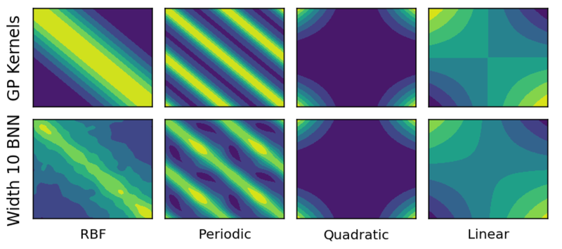
Comparability of Gram matrices between true GP kernels (high row) and their width 10 neural community approximations (backside row).
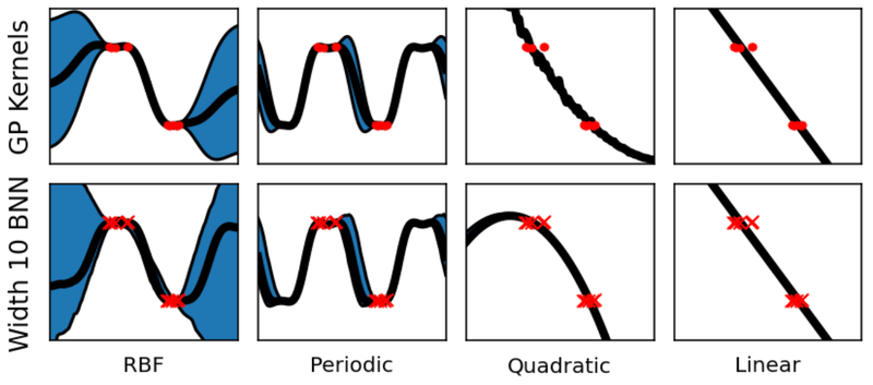
Comparability of regression outcomes between true GP kernels (high row) and their width 10 neural community approximations (backside row).
Lastly, the interpretation is accomplished with BNN analogues of the Addition and Multiplication operators over GPs, and enter warping to supply periodic kernels. BNN addition is straightforwardly given by including the outputs of the element BNNs. BNN multiplication is achieved by multiplying the activations of the hidden layers of the BNNs after which making use of a shared dense layer. We’re subsequently restricted to solely multiplying BNNs with the identical hidden width.
Utilizing AutoBNN
The AutoBNN bundle is accessible inside Tensorflow Likelihood. It’s applied in JAX and makes use of the flax.linen neural community library. It implements all the base kernels and operators mentioned to this point (Linear, Quadratic, Matern, ExponentiatedQuadratic, Periodic, Addition, Multiplication) plus one new kernel and three new operators:
- a
OneLayerkernel, a single hidden layer ReLU BNN, - a
ChangePointoperator that enables easily switching between two kernels, - a
LearnableChangePointoperator which is similar asChangePointbesides place and slope are given prior distributions and might be learnt from the info, and - a
WeightedSumoperator.
WeightedSum combines two or extra BNNs with learnable mixing weights, the place the learnable weights observe a Dirichlet prior. By default, a flat Dirichlet distribution with focus 1.0 is used.
WeightedSums permit a “gentle” model of construction discovery, i.e., coaching a linear mixture of many potential fashions without delay. In distinction to construction discovery with discrete constructions, similar to in AutoGP, this permits us to make use of commonplace gradient strategies to study constructions, moderately than utilizing costly discrete optimization. As a substitute of evaluating potential combinatorial constructions in sequence, WeightedSum permits us to judge them in parallel.
To simply allow exploration, AutoBNN defines a variety of mannequin constructions that include both top-level or inside WeightedSums. The names of those fashions can be utilized as the primary parameter in any of the estimator constructors, and embody issues like sum_of_stumps (the WeightedSum over all the bottom kernels) and sum_of_shallow (which provides all potential mixtures of base kernels with all operators).
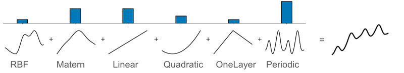
Illustration of the sum_of_stumps mannequin. The bars within the high row present the quantity by which every base kernel contributes, and the underside row reveals the operate represented by the bottom kernel. The ensuing weighted sum is proven on the proper.
The determine beneath demonstrates the strategy of construction discovery on the N374 (a time sequence of yearly monetary information ranging from 1949) from the M3 dataset. The six base constructions had been ExponentiatedQuadratic (which is similar because the Radial Foundation Perform kernel, or RBF for brief), Matern, Linear, Quadratic, OneLayer and Periodic kernels. The determine reveals the MAP estimates of their weights over an ensemble of 32 particles. The entire excessive chance particles gave a big weight to the Periodic element, low weights to Linear, Quadratic and OneLayer, and a big weight to both RBF or Matern.
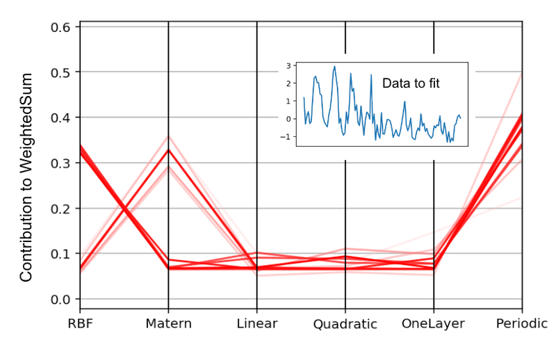
Parallel coordinates plot of the MAP estimates of the bottom kernel weights over 32 particles. The sum_of_stumps mannequin was educated on the N374 sequence from the M3 dataset (insert in blue). Darker strains correspond to particles with increased likelihoods.
By utilizing WeightedSums because the inputs to different operators, it’s potential to precise wealthy combinatorial constructions, whereas holding fashions compact and the variety of learnable weights small. For example, we embody the sum_of_products mannequin (illustrated within the determine beneath) which first creates a pairwise product of two WeightedSums, after which a sum of the 2 merchandise. By setting among the weights to zero, we are able to create many various discrete constructions. The overall variety of potential constructions on this mannequin is 216, since there are 16 base kernels that may be turned on or off. All these constructions are explored implicitly by coaching simply this one mannequin.
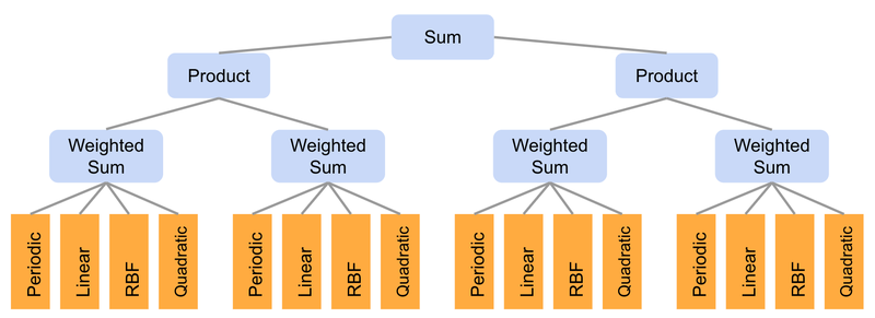
Illustration of the “sum_of_products” mannequin. Every of the 4 WeightedSums have the identical construction because the “sum_of_stumps” mannequin.
We’ve got discovered, nevertheless, that sure mixtures of kernels (e.g., the product of Periodic and both the Matern or ExponentiatedQuadratic) result in overfitting on many datasets. To forestall this, we’ve outlined mannequin lessons like sum_of_safe_shallow that exclude such merchandise when performing construction discovery with WeightedSums.
For coaching, AutoBNN gives AutoBnnMapEstimator and AutoBnnMCMCEstimator to carry out MAP and MCMC inference, respectively. Both estimator might be mixed with any of the six chance features, together with 4 based mostly on regular distributions with completely different noise traits for steady information and two based mostly on the unfavourable binomial distribution for depend information.
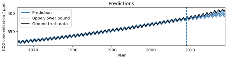
Outcome from operating AutoBNN on the Mauna Loa CO2 dataset in our instance colab. The mannequin captures the pattern and seasonal element within the information. Extrapolating into the long run, the imply prediction barely underestimates the precise pattern, whereas the 95% confidence interval steadily will increase.
To suit a mannequin like within the determine above, all it takes is the next 10 strains of code, utilizing the scikit-learn–impressed estimator interface:
import autobnn as ab

mannequin = ab.operators.Add(
    bnns=(ab.kernels.PeriodicBNN(width=50),
          ab.kernels.LinearBNN(width=50),
          ab.kernels.MaternBNN(width=50)))

estimator = ab.estimators.AutoBnnMapEstimator(
    mannequin, 'normal_likelihood_logistic_noise', jax.random.PRNGKey(42),
    durations=[12])

estimator.match(my_training_data_xs, my_training_data_ys)
low, mid, excessive = estimator.predict_quantiles(my_training_data_xs)
Conclusion
AutoBNN gives a robust and versatile framework for constructing refined time sequence prediction fashions. By combining the strengths of BNNs and GPs with compositional kernels, AutoBNN opens a world of potentialities for understanding and forecasting complicated information. We invite the neighborhood to attempt the colab, and leverage this library to innovate and clear up real-world challenges.
Acknowledgements
AutoBNN was written by Colin Carroll, Thomas Colthurst, Urs Köster and Srinivas Vasudevan. We wish to thank Kevin Murphy, Brian Patton and Feras Saad for his or her recommendation and suggestions.
AutoBNN combines the interpretability of conventional probabilistic approaches with the scalability and adaptability of neural networks for constructing refined time sequence prediction fashions utilizing complicated information.
Time sequence issues are ubiquitous, from forecasting climate and site visitors patterns to understanding financial developments. Bayesian approaches begin with an assumption concerning the information’s patterns (prior likelihood), accumulating proof (e.g., new time sequence information), and repeatedly updating that assumption to type a posterior likelihood distribution. Conventional Bayesian approaches like Gaussian processes (GPs) and Structural Time Collection are extensively used for modeling time sequence information, e.g., the generally used Mauna Loa CO2 dataset. Nevertheless, they usually depend on area consultants to painstakingly choose applicable mannequin elements and could also be computationally costly. Options similar to neural networks lack interpretability, making it obscure how they generate forecasts, and do not produce dependable confidence intervals.
To that finish, we introduce AutoBNN, a brand new open-source bundle written in JAX. AutoBNN automates the invention of interpretable time sequence forecasting fashions, gives high-quality uncertainty estimates, and scales successfully to be used on giant datasets. We describe how AutoBNN combines the interpretability of conventional probabilistic approaches with the scalability and adaptability of neural networks.
AutoBNN
AutoBNN relies on a line of analysis that over the previous decade has yielded improved predictive accuracy by modeling time sequence utilizing GPs with discovered kernel constructions. The kernel operate of a GP encodes assumptions concerning the operate being modeled, such because the presence of developments, periodicity or noise. With discovered GP kernels, the kernel operate is outlined compositionally: it’s both a base kernel (similar to Linear, Quadratic, Periodic, Matérn or ExponentiatedQuadratic) or a composite that mixes two or extra kernel features utilizing operators similar to Addition, Multiplication, or ChangePoint. This compositional kernel construction serves two associated functions. First, it’s easy sufficient {that a} consumer who’s an professional about their information, however not essentially about GPs, can assemble an inexpensive prior for his or her time sequence. Second, strategies like Sequential Monte Carlo can be utilized for discrete searches over small constructions and may output interpretable outcomes.
AutoBNN improves upon these concepts, changing the GP with Bayesian neural networks (BNNs) whereas retaining the compositional kernel construction. A BNN is a neural community with a likelihood distribution over weights moderately than a hard and fast set of weights. This induces a distribution over outputs, capturing uncertainty within the predictions. BNNs convey the next benefits over GPs: First, coaching giant GPs is computationally costly, and conventional coaching algorithms scale because the dice of the variety of information factors within the time sequence. In distinction, for a hard and fast width, coaching a BNN will usually be roughly linear within the variety of information factors. Second, BNNs lend themselves higher to GPU and TPU {hardware} acceleration than GP coaching operations. Third, compositional BNNs might be simply mixed with conventional deep BNNs, which have the power to do function discovery. One might think about “hybrid” architectures, by which customers specify a top-level construction of Add(Linear, Periodic, Deep), and the deep BNN is left to study the contributions from doubtlessly high-dimensional covariate info.
How may one translate a GP with compositional kernels right into a BNN then? A single layer neural community will usually converge to a GP because the variety of neurons (or “width”) goes to infinity. Extra not too long ago, researchers have found a correspondence within the different path — many standard GP kernels (similar to Matern, ExponentiatedQuadratic, Polynomial or Periodic) might be obtained as infinite-width BNNs with appropriately chosen activation features and weight distributions. Moreover, these BNNs stay near the corresponding GP even when the width may be very a lot lower than infinite. For instance, the figures beneath present the distinction within the covariance between pairs of observations, and regression outcomes of the true GPs and their corresponding width-10 neural community variations.
Comparability of Gram matrices between true GP kernels (high row) and their width 10 neural community approximations (backside row).
Comparability of regression outcomes between true GP kernels (high row) and their width 10 neural community approximations (backside row).
Lastly, the interpretation is accomplished with BNN analogues of the Addition and Multiplication operators over GPs, and enter warping to supply periodic kernels. BNN addition is straightforwardly given by including the outputs of the element BNNs. BNN multiplication is achieved by multiplying the activations of the hidden layers of the BNNs after which making use of a shared dense layer. We’re subsequently restricted to solely multiplying BNNs with the identical hidden width.
Utilizing AutoBNN
The AutoBNN bundle is accessible inside Tensorflow Likelihood. It’s applied in JAX and makes use of the flax.linen neural community library. It implements all the base kernels and operators mentioned to this point (Linear, Quadratic, Matern, ExponentiatedQuadratic, Periodic, Addition, Multiplication) plus one new kernel and three new operators:
- a
OneLayerkernel, a single hidden layer ReLU BNN, - a
ChangePointoperator that enables easily switching between two kernels, - a
LearnableChangePointoperator which is similar asChangePointbesides place and slope are given prior distributions and might be learnt from the info, and - a
WeightedSumoperator.
WeightedSum combines two or extra BNNs with learnable mixing weights, the place the learnable weights observe a Dirichlet prior. By default, a flat Dirichlet distribution with focus 1.0 is used.
WeightedSums permit a “gentle” model of construction discovery, i.e., coaching a linear mixture of many potential fashions without delay. In distinction to construction discovery with discrete constructions, similar to in AutoGP, this permits us to make use of commonplace gradient strategies to study constructions, moderately than utilizing costly discrete optimization. As a substitute of evaluating potential combinatorial constructions in sequence, WeightedSum permits us to judge them in parallel.
To simply allow exploration, AutoBNN defines a variety of mannequin constructions that include both top-level or inside WeightedSums. The names of those fashions can be utilized as the primary parameter in any of the estimator constructors, and embody issues like sum_of_stumps (the WeightedSum over all the bottom kernels) and sum_of_shallow (which provides all potential mixtures of base kernels with all operators).
Illustration of the sum_of_stumps mannequin. The bars within the high row present the quantity by which every base kernel contributes, and the underside row reveals the operate represented by the bottom kernel. The ensuing weighted sum is proven on the proper.
The determine beneath demonstrates the strategy of construction discovery on the N374 (a time sequence of yearly monetary information ranging from 1949) from the M3 dataset. The six base constructions had been ExponentiatedQuadratic (which is similar because the Radial Foundation Perform kernel, or RBF for brief), Matern, Linear, Quadratic, OneLayer and Periodic kernels. The determine reveals the MAP estimates of their weights over an ensemble of 32 particles. The entire excessive chance particles gave a big weight to the Periodic element, low weights to Linear, Quadratic and OneLayer, and a big weight to both RBF or Matern.
Parallel coordinates plot of the MAP estimates of the bottom kernel weights over 32 particles. The sum_of_stumps mannequin was educated on the N374 sequence from the M3 dataset (insert in blue). Darker strains correspond to particles with increased likelihoods.
By utilizing WeightedSums because the inputs to different operators, it’s potential to precise wealthy combinatorial constructions, whereas holding fashions compact and the variety of learnable weights small. For example, we embody the sum_of_products mannequin (illustrated within the determine beneath) which first creates a pairwise product of two WeightedSums, after which a sum of the 2 merchandise. By setting among the weights to zero, we are able to create many various discrete constructions. The overall variety of potential constructions on this mannequin is 216, since there are 16 base kernels that may be turned on or off. All these constructions are explored implicitly by coaching simply this one mannequin.
Illustration of the “sum_of_products” mannequin. Every of the 4 WeightedSums have the identical construction because the “sum_of_stumps” mannequin.
We’ve got discovered, nevertheless, that sure mixtures of kernels (e.g., the product of Periodic and both the Matern or ExponentiatedQuadratic) result in overfitting on many datasets. To forestall this, we’ve outlined mannequin lessons like sum_of_safe_shallow that exclude such merchandise when performing construction discovery with WeightedSums.
For coaching, AutoBNN gives AutoBnnMapEstimator and AutoBnnMCMCEstimator to carry out MAP and MCMC inference, respectively. Both estimator might be mixed with any of the six chance features, together with 4 based mostly on regular distributions with completely different noise traits for steady information and two based mostly on the unfavourable binomial distribution for depend information.
Outcome from operating AutoBNN on the Mauna Loa CO2 dataset in our instance colab. The mannequin captures the pattern and seasonal element within the information. Extrapolating into the long run, the imply prediction barely underestimates the precise pattern, whereas the 95% confidence interval steadily will increase.
To suit a mannequin like within the determine above, all it takes is the next 10 strains of code, utilizing the scikit-learn–impressed estimator interface:
import autobnn as ab

mannequin = ab.operators.Add(
    bnns=(ab.kernels.PeriodicBNN(width=50),
          ab.kernels.LinearBNN(width=50),
          ab.kernels.MaternBNN(width=50)))

estimator = ab.estimators.AutoBnnMapEstimator(
    mannequin, 'normal_likelihood_logistic_noise', jax.random.PRNGKey(42),
    durations=[12])

estimator.match(my_training_data_xs, my_training_data_ys)
low, mid, excessive = estimator.predict_quantiles(my_training_data_xs)
Conclusion
AutoBNN gives a robust and versatile framework for constructing refined time sequence prediction fashions. By combining the strengths of BNNs and GPs with compositional kernels, AutoBNN opens a world of potentialities for understanding and forecasting complicated information. We invite the neighborhood to attempt the colab, and leverage this library to innovate and clear up real-world challenges.
Acknowledgements
AutoBNN was written by Colin Carroll, Thomas Colthurst, Urs Köster and Srinivas Vasudevan. We wish to thank Kevin Murphy, Brian Patton and Feras Saad for his or her recommendation and suggestions.


