


All code used on this article is offered on GitHub. The enterprise logic and modeling features are situated within the
src/choicelisting, particularly within the following file:
src/modeling/score_computation.pyThe corresponding evaluation and outcomes are documented in:
09_score_computation.qmdThe photographs, tables, and charts had been generated with the assistance of the Codex coding assistant.
, your credit score rating follows you in every single place. It decides if you happen to get a mortgage, a bank card, and even an residence. The mannequin behind most of those choices is FICO. Its logic is straightforward when you break it down.
FICO weighs 5 issues:
- Cost historical past (35%): pay your payments on time.
- Quantities owed (30%): hold your credit score use beneath 20%.
- Size of historical past (15%): the longer, the higher.
- Credit score combine (10%): use several types of credit score.
- New credit score (10%): restrict new functions.
In the event you pay your bank card payments on time, your rating rises. Cost historical past carries essentially the most weight.
These weights produce a rating, break up into ranges:
- 300–579: Poor.
- 580–669: Truthful.
- 670–739: Good.
- 740–799: Very Good.
- 800–850: Glorious.
This text follows the identical logic, however applies it to our personal mannequin.
We use the dataset from this sequence on constructing a scoring mannequin. The objective is straightforward: give every retained variable a weight, compute the rating for each shopper in our knowledge, and present how a brand new shopper’s rating is calculated.
As earlier than, Codex helped write the code and construct the tables and charts. I hold saying this as a result of it issues: you should use AI brokers to hurry up your work. However examine their output. Belief grows solely whenever you confirm it. Use these instruments, however keep alert.
Let’s recall what we discovered final time. We saved 4 variables:
loan_int_rate: the mortgage’s rate of interest.loan_percent_income: the share of revenue spent on mortgage funds.cb_person_default_on_file: whether or not the borrower defaulted earlier than.home_ownership_3: the borrower’s housing standing.

Like FICO, we give every variable a weight and construct a rating from 0 to 1000. A excessive rating means low threat. A low rating means excessive threat of default.
From Mannequin Coefficients to a Rating
We flip every coefficient right into a rating.
Rating for every class of a variable
Take loan_int_rate for instance. The rating for class is:
Right here, is the coefficient for class of variable . And is the best coefficient for variable . For instance, for the variable loan_int_rate, the best coefficient is .
This method provides the rating desk beneath.

A shopper’s rating, step-by-step
Take a brand new shopper. We examine which class they fall into for every variable:
loan_int_rateis 10%. Rating: 181.72.loan_percent_incomeis 25%. Rating: 0.- No previous default (
cb_person_default_on_file = N). Rating: 59.52. - Owns their residence (
home_ownership_3 = OWN). Rating: 373.94.
We add these scores to get the ultimate rating for the shopper:
We repeat this for each shopper in our knowledge.
How A lot Every Variable Issues
As soon as we have now the rating, we ask: which variable drives it most?
We measure this on the coaching knowledge:

Right here:
- The bar over represents the typical rating of variable j, weighted by inhabitants;
In plain phrases, exhibits how a lot variable strikes the rating. The better the variation amongst its totally different classes, the upper its weight.
The desk beneath exhibits every variable’s weight.

loan_percent_income weighs essentially the most, at 35%. Then home_ownership_3 at 31%, loan_int_rate at 28%, and cb_person_default_on_file final.
This is sensible. A shopper who spends greater than 20% of their revenue on mortgage funds is dangerous. The truth that this variable drives the rating essentially the most is sweet information: the mannequin picks up the fitting sign.
Does the Rating Separate Danger Nicely?
Earlier than we construct the chance grid, we examine if the rating does its job: break up defaulters from non-defaulters.
We plot the rating’s density for every group, break up by default, throughout prepare, check, and out-of-time knowledge.

The additional aside the 2 curves, the higher the rating works.
What we see: defaults cluster at low scores. Non-defaults cluster at excessive scores. That is what we wish: excessive rating, low threat.
Constructing the Danger Grid
Now we construct the grid.
Step 1: Default fee by rating group
We break up the rating into 20 equal teams and plot the default fee for every. We begin by plotting the default fee towards the vingtiles (20 equal-sized segments) of the ultimate rating.

This chart is the muse for the grid: it provides a pure place to begin for grouping the 20 segments into six threat lessons.
Step 2: Six threat lessons
Primarily based on the chart, we group the 20 segments like this:
- Teams 1, 2, 3, with scores between 0 and 241: lowest scores, highest threat.
- Teams 4, 5, 6, with scores between 241 and 331.
- Teams 7, 8, with scores between 332 and 498.
- Teams 9, 10, 11, 12, with scores between 498 and 589.
- Teams 13, 14, 15, 16, 17, with scores between 589 and 780.
- Teams 18, 19, 20, with scores between 781 and 1000: highest scores, lowest threat.

These lessons should meet three guidelines:
✓ Every class should be uniform in threat;
✓ Every class should differ from the following by at the very least 30%;
✓ Every class should maintain at the very least 1% of all purchasers.

The desk above exhibits that these guidelines are being adopted.
Step 3: Checking stability
A threat grid solely works if it holds up over time. We examine two issues:
- Riskier lessons should at all times present greater default charges, throughout the complete historical past.
- The variety of purchasers in every class should keep regular over time.


Each maintain true: threat stays in the fitting order, and sophistication sizes keep regular.
Conclusion
This text closes our sequence on constructing a scoring mannequin. We began with the information and finish with a threat grid.
We constructed a rating from 0 to 1000 by scoring every class of every variable. A shopper’s rating is the sum of those class scores. The rating splits threat nicely: defaulters and non-defaulters land in clearly totally different ranges.
Every variable’s weight: loan_percent_income leads at 35%, then home_ownership_3 at 31%, loan_int_rate at 28%, and cb_person_default_on_file final.
👉 Good to know: the upper your revenue in comparison with your mortgage, the upper your rating.
The ultimate threat grid:
- 0–241: Very Excessive Danger.
- 241–331: Excessive Danger.
- 332–498: Medium-Excessive Danger.
- 499–589: Medium Danger.
- 590–789: Low Danger.
- 790–1000: Very Low Danger.
I saved this text brief on function. We constructed the grid right here utilizing vingtiles and visible grouping, however different statistical strategies exist to separate scores into homogeneous lessons. Okay-means, hierarchical clustering, and Weight of Proof (WoE) all provide a extra rigorous path to the identical objective. That would be the topic of my subsequent article.
References
[1] Lorenzo Beretta and Alessandro Santaniello.
Nearest Neighbor Imputation Algorithms: A Important Analysis.
Nationwide Library of Medication, 2016.
[2] Nexialog Consulting.
Traitement des données manquantes dans le milieu bancaire.
Working paper, 2022.
[3] John T. Hancock and Taghi M. Khoshgoftaar.
Survey on Categorical Information for Neural Networks.
Journal of Massive Information, 7(28), 2020.
[4] Melissa J. Azur, Elizabeth A. Stuart, Constantine Frangakis, and Philip J. Leaf.
A number of Imputation by Chained Equations: What Is It and How Does It Work?
Worldwide Journal of Strategies in Psychiatric Analysis, 2011.
[5] Majid Sarmad.
Sturdy Information Evaluation for Factorial Experimental Designs: Improved Strategies and Software program.
Division of Mathematical Sciences, College of Durham, England, 2006.
[6] Daniel J. Stekhoven and Peter Bühlmann.
MissForest—Non-Parametric Lacking Worth Imputation for Combined-Sort Information.Bioinformatics, 2011.
[7] Supriyanto Wibisono, Anwar, and Amin.
Multivariate Climate Anomaly Detection Utilizing the DBSCAN Clustering Algorithm.
Journal of Physics: Convention Sequence, 2021.
[8] Laborda, J., & Ryoo, S. (2021). Characteristic choice in a credit score scoring mannequin. Arithmetic, 9(7), 746.
Information & Licensing
The dataset used on this article is licensed below the Artistic Commons Attribution 4.0 Worldwide (CC BY 4.0) license.
This license permits anybody to share and adapt the dataset for any function, together with industrial use, offered that correct attribution is given to the supply.
For extra particulars, see the official license textual content: CC0: Public Area.
Disclaimer
Any remaining errors or inaccuracies are the creator’s accountability. Suggestions and corrections are welcome.


