How I Constructed a Multi-Agent System for Interrupted Time Collection Evaluation (ITSA)

One month in the past your organization determined to launch a model new checkout course of. The choice speculation was quite simple: a three-step checkout would drive extra purchases and income than the earlier one-step checkout, primarily based on trade benchmarks and good UX/UI practices.

Simply to ensure this resolution actually strikes the needle (and with the intention of quantifying it), you recommended that an A/B check can be the very best answer to measure the impact and reject the null speculation. The end result: you couldn’t persuade the stakeholders to run a correctly designed A/B check and the choice of launching this new checkout was made anyway.

Nonetheless, one month later, proper now, these stakeholders ask questions resembling: “what’s the impact of the brand new checkout?” “Did it work?” or “Did we lose cash with it?”… I’m very certain that the majority of you may have been on this state of affairs and may know some quasi-experimental strategies resembling Distinction-in-differences or Artificial Management Strategies however… what are you able to do when there are not any different markets to check towards, and the corporate is not sufficiently big to construct a reputable artificial management group?

I need to introduce ITSA (Interrupted Time Collection Evaluation), a way I’ve been utilizing over the past 4 years in conditions the place you possibly can’t run a randomized management trial and you’ve got few choices between all the huge quantity of strategies associated to observational research. Additionally, I’ll introduce how we created a multi-agent system to run ITSA, the architectural, statistical and software program selections (and trade-offs) we would have liked to make to develop this knowledge product and the advantages this answer affords.

ITSA and why it issues

A quick introduction

Measurement in digital enterprise has lengthy trusted the pre- versus post-intervention strategy for precisely these conditions. I am certain you have heard one thing like: “simply examine what occurred after the change with the interval earlier than.” Perhaps you have even believed it is a good strategy. Respectfully, let me present you why it falls quick.

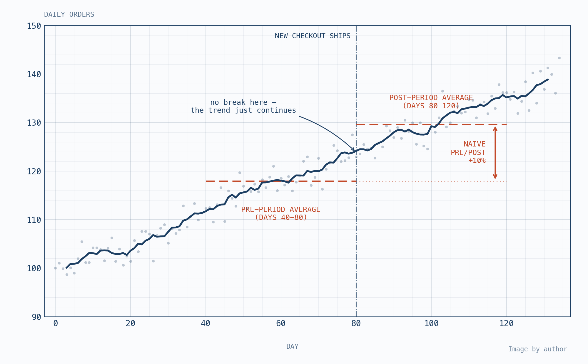
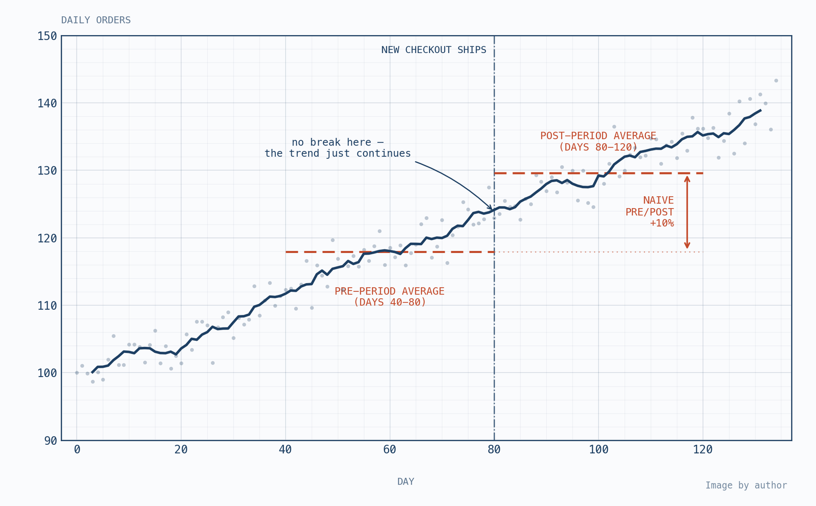
Simulated day by day orders climb steadily from about 100 to 140 over 130 days. A brand new checkout ships on day 80, however the collection exhibits no break: the upward pattern merely continues. Evaluating the pre-period common (days 40–80) with the post-period common (days 80–120) suggests a +10% carry that the checkout did not trigger; the pre-existing pattern did. That is the naive pre/publish entice that Interrupted Time Collection Evaluation (ITSA) is designed to keep away from.

From a statistical standpoint, evaluating the imply earlier than and after the intervention is a naive strategy: it ignores pre-existing tendencies and seasonality, doesn’t account for autocorrelation when quantifying uncertainty, and can’t distinguish the intervention from concurrent shocks. Within the Determine 1 state of affairs, this comparability would lead you to conclude that the intervention elevated day by day orders by 10%. And also you’d be unsuitable.

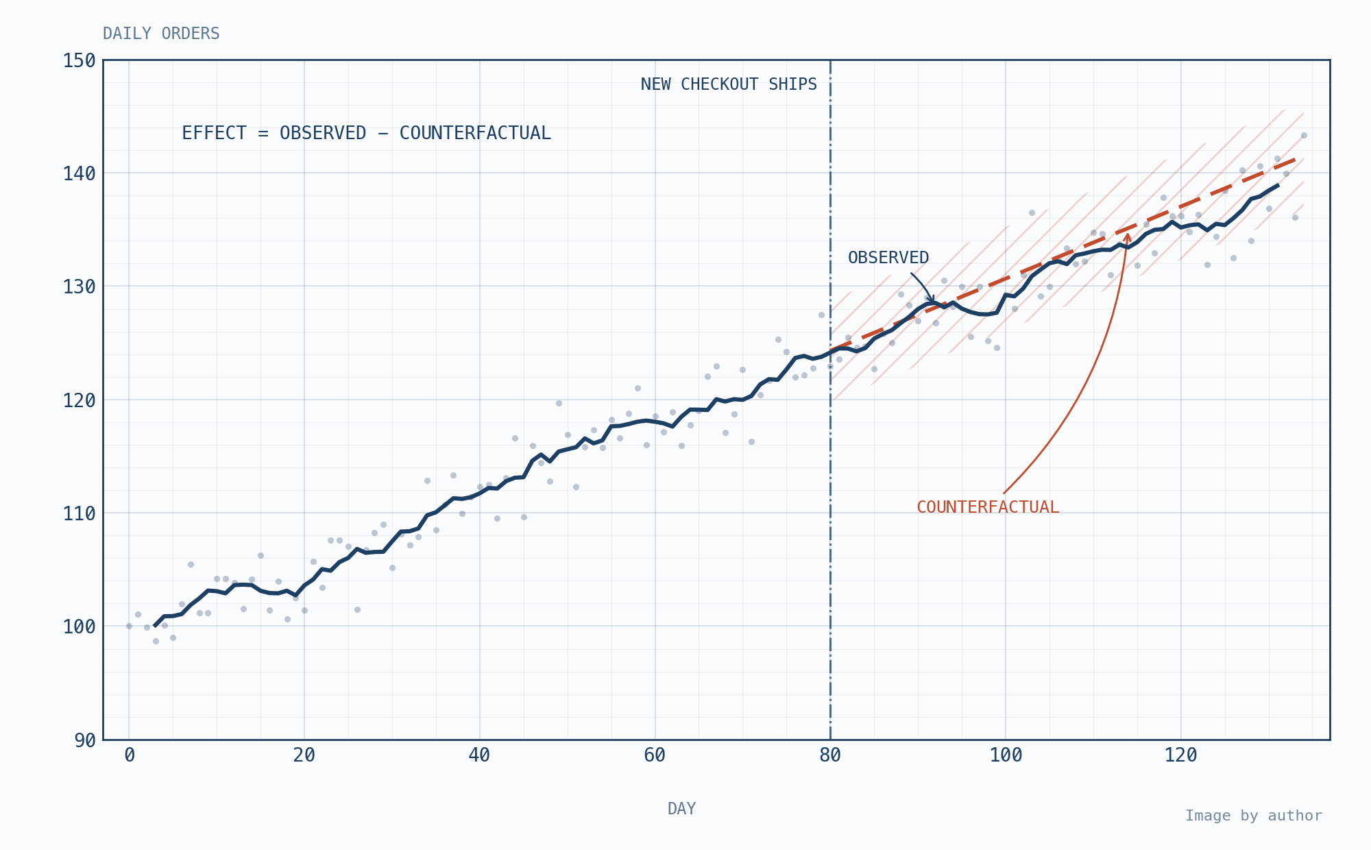
The identical simulated day by day orders collection, now analysed with a counterfactual. After the brand new checkout ships on day 80, the pre-intervention pattern is projected ahead as a dashed line with an uncertainty band: what would have occurred with out the change. Noticed orders keep inside that band, so the estimated impact is basically zero. In Interrupted Time Collection Evaluation, the impact is the hole between the noticed collection and the counterfactual, not between the pre and publish averages.

In Determine 2 you possibly can see a unique strategy: as a substitute of evaluating the typical worth from pre and post-intervention, you possibly can examine what occurred post-intervention (Noticed) with what would have occurred if we hadn’t launched the three-step checkout (Counterfactual). On this case there isn’t a optimistic or unfavorable impact attributed to our intervention. Why? as a result of the impact is measured by subtracting the counterfactual from the noticed worth.

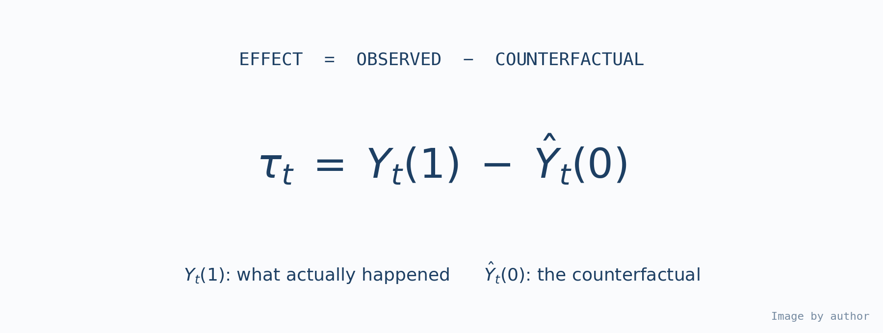
The potential-outcomes definition of the impact: τ_t = Y_t(1) − Ŷ_t(0). Y_t(1) is what truly occurred after the intervention; Ŷ_t(0) is the estimated counterfactual, what would have occurred with out it. Each causal inference technique, together with Interrupted Time Collection Evaluation, differs primarily in the way it estimates that counterfactual.

How will you estimate the counterfactual? Nicely, that’s the entire level: it depends upon the identification and estimation method you utilize. You need to use Distinction-in-difference in the event you can assume parallel tendencies, you should use Artificial Management Strategies in the event you can construct a correctly weighted artificial management group, and so forth.

ITSA makes use of a unique strategy: it makes use of the end result’s personal pre-intervention trajectory to estimate what would’ve occurred after the intervention in its absence. In its easiest type, a segmented regression estimates the baseline degree and the pre-existing pattern, then tasks that trajectory into the post-intervention interval. The intervention impact is just not the distinction between the post- and pre-intervention durations, however the distinction between the noticed post-intervention trajectory and this projected counterfactual.

ITSA assumptions and when to make use of it (and once you should not)

This technique has its personal assumptions, and you could know them earlier than utilizing it to make the very best resolution attainable. In a nutshell, listed here are the ten most essential assumptions when utilizing ITSA:

1. Counterfactual continuity: Absent the intervention, the pre-intervention pattern would have continued unchanged. Extrapolating that pattern is the counterfactual in a single-group design. That is the belief that carries all the load and it’s basically untestable, because you by no means observe the world with out the intervention. It clearly connects with the basic downside of causal inference.

2. You want a transparent, identified intervention level. It means you want a well-defined onset date.

3. No co-interventions or concurrent shocks at T0 (the historical past risk). Linden explicitly warns about a number of coverage shifts across the intervention.

4. No anticipation. The intervention doesn’t have an effect on the pre-intervention interval.

5. Any time-varying confounder should evolve easily, so it stays distinguishable from the sharp leap of the intervention. An abrupt confounder masquerades as an impact.

6. Seasonality and cycles are managed for (day-of-week, month, recurring campaigns).

7. Sufficient equally-spaced observations earlier than and after. Widespread rule of thumb: ≥8 factors per phase. With out sufficient observations, the minimal detectable impact (MDE) rises above the true impact and you will not detect it.

8. Autocorrelation is dealt with. Time-series errors are serially correlated. Ignoring it produces miscalibrated customary errors and confidence intervals.

9. Constant consequence measurement over time. The metric’s definition and assortment do not change throughout pre-intervention and post-intervention durations.

10. The underlying regression mannequin’s personal assumptions maintain.

In a nuthell, ITSA assumes that, with out he intervention:

• The pre-intervention data-generating course of would have continued into the post-intervention interval.

• No concurrent occasion can clarify the noticed interruption.

• The intervention timing and anticipated affect sample are accurately specified.

• Final result measurement stays secure.

• Pattern, seasonality and residual dependence are adequately modelled.

When to make use of ITSA, then? Attain for it when three circumstances line up directly, and once they do, it’s typically the very best device accessible, not a comfort prize.

1. You could not randomize. The change was shipped to everybody directly: a brand new checkout, a pricing replace, an search engine optimization migration. There isn’t any untreated group of customers to check towards, so an A/B check is off the desk (which is strictly how we acquired right here).

2. You haven’t any credible management group. No parallel market, area, or product line that behaved like yours however by no means acquired the change. That is what guidelines out difference-in-differences and artificial management: each want a comparability unit, and you do not have one. ITSA is the single-group design as a result of it builds the counterfactual from your personal historical past as a substitute.

3. You have got a clear time collection. One constantly measured consequence, at common intervals, with sufficient observations each earlier than and after a clearly dated intervention.

ITSA is healthier understood as a analysis design than as a single estimation method and it shouldn’t be chosen merely as a result of you may have a time collection and an intervention date. If the intervention timing is ambiguous, the pre-intervention interval is already contaminated, one other related occasion happens round T0, or the collection supplies too little temporal help, a extra refined mannequin is not going to rescue the identification technique.

Why a multi-agent system to run ITSA?

We began working Interrupted Time Collection Evaluation in 2023. We discovered that this system might convey extra details about the true impact of an intervention. In our case, we attempt to optimize consumer expertise and conversions by on-line experimentation and one query we heard typically was: “the impact at this AB check is that this one, okay, however will I see this uplift if I launch this new model?”

That’s a really troublesome query as a result of you possibly can’t reply this with one other AB check and as I defined firstly, DiD, RDD and SCM aren’t all the time possible both, so we needed to search for alternate options. That’s after we discovered ITSA.

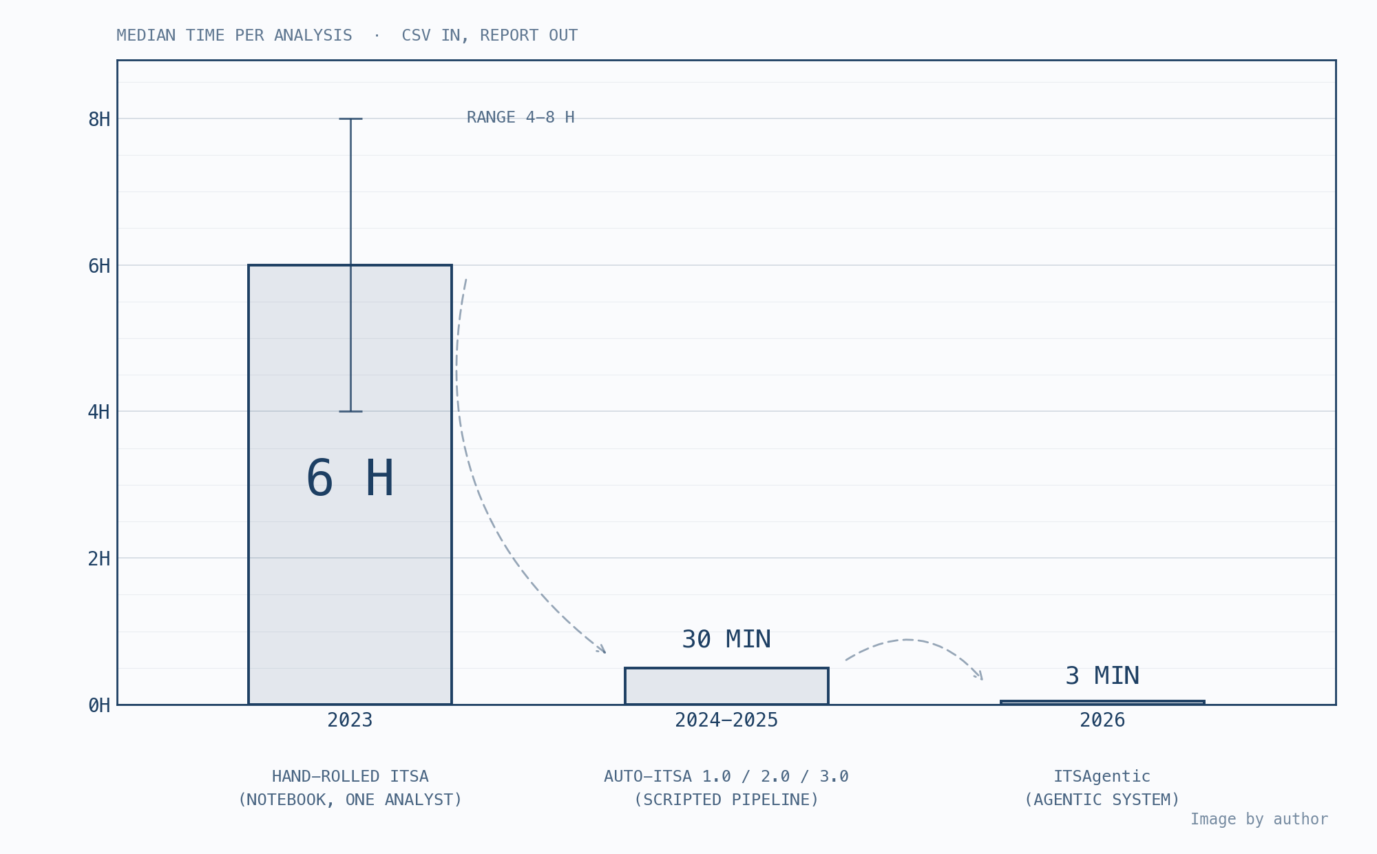
Median time to run one Interrupted Time Collection Evaluation, from CSV in to report out. In 2023, a hand-rolled evaluation in a pocket book took a median of 6 hours (vary 4–8 hours). Auto-ITSA 1.0–3.0, a scripted Python pipeline utilized in 2024–2025, minimize it to half-hour. ITSAgentic, the multi-agent system launched in 2026, brings it down to three minutes.

As I stated, we began on this in 2023 and we spent 6 hours (medians imputed from our online-experimentation group’s time logs) each time we would have liked to run this type of evaluation. That wasn’t very productive and I made a decision to create an inner pipeline (known as Auto-ITSA) for univariate and multivariate evaluation.

Auto-ITSA was principally an inner device inbuilt Python that acquired the info and primarily based on completely different parameters (intervention date, knowledge sort, the character of the intervention…) was capable of robotically decide the very best statistical strategy (OLS, WLS, Unfavorable Binomial…) to create the very best counterfactual. The end result: With this pipeline we improved and standardized ITS evaluation and minimize it from 6 hours to half-hour per evaluation.

However here is the factor: we needed to enhance Auto-ITSA by including extra visible graphs, extra flexibility in numerous situations, extra libraries and approaches… We have been getting important positive factors in technical and statistical phrases however dropping in time-to-value: the parametrization in Auto-ITSA 3.0 was time-consuming and wanted increasingly statistical information in each new iteration. That was the 0-day of ITSAgentic.

ITSAgentic: an AI product to run Interrupted Time Collection Evaluation

At first of 2026 I made a decision to create ITSAgentic attributable to the truth that the reasoning capabilities of LLMs in November of 2025 made a glow-up. I began with this schema to work out what I wanted to construct.

In a nutshell, ITSAgentic is an AI product that takes an enter (a dataframe, for instance) together with the parameters that outline the intervention: the intervention date, the metric sort, the publicity share (step, ramp, pulse or decay), and so forth. From there, every little thing is a sequence of selections about which evaluation to run and what its end result means.

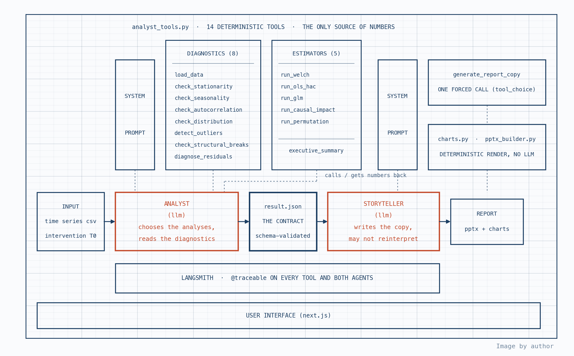
ITSAgentic structure. A time collection CSV and an intervention date go to the analyst agent, an LLM that chooses which analyses to run and reads the diagnostics. Each quantity comes from 14 deterministic Python instruments: 8 diagnostics and 5 estimators, plus an govt abstract. The analyst writes a schema-validated end result.json, the one contract between brokers. The storyteller agent reads it and makes one pressured name to jot down the report copy, which deterministic chart and PPTX builders render. LangSmith traces each device and each brokers, behind a Subsequent.js interface.

The primary agent is a quantitative analyst. It really works by a prescribed order (load_data, check_stationarity, check_seasonality, check_autocorrelation, and so forth) after which picks the first estimator that matches what these diagnostics discovered: OLS-HAC and GLM-NB, amongst others. However here is the important thing design resolution: the mannequin by no means computes a single quantity.

All 14 instruments are plain Python (statsmodels, scipy, pandas), and they’re deterministic by development: the identical enter returns the identical output, each time, with or with out an LLM within the room. What I needed from the mannequin was reasoning about the output, not the output itself. Choosing the proper estimator for a non-stationary rely collection with weekly seasonality is a judgement name. Computing its coefficients is arithmetic, and arithmetic is the very last thing you need an LLM doing.

The analyst finishes with an executive_summary: the impact and its uncertainty, the warnings that apply, a confidence degree, and a advisable motion drawn from a closed vocabulary (an uplift that is not statistically important, a roll-out to extra markets, stopping the intervention as a result of the first metric dropped, and so forth). That abstract is not prose. It is a schema-validated JSON file, end result.json, and it’s the solely factor that crosses the road between the 2 brokers.

The storyteller is the second agent inside ITSAgentic, and it is the one which turns a statistical end result into the story a stakeholder truly reads. Making it a separate agent was a deliberate resolution, not an architectural accident. It has its personal identification (it is the individual presenting to the enterprise) its personal base immediate, and its personal set of instruments, which don’t have anything to do with statistics: chart technology and slide constructing, so the output is a completed presentation fairly than a wall of textual content. They share nearly no tooling and no tone, so I break up them.

And there is a second purpose to separate them, which is the one I care most about: the storyteller cannot invent something. It by no means sees the dataframe, by no means sees the uncooked device output, and by no means runs a mannequin. It receives end result.json and makes precisely one pressured name to show it into stakeholder-facing copy. It can not recompute an impact, improve a “no important impact” right into a win, or quietly drop a warning that spoils the narrative, as a result of none of these numbers are inside its attain. Every little thing it could say, it has to say utilizing what the analyst already dedicated to in writing.

The significance of publicity share

Textbook ITSA codes the intervention as a 0/1 dummy: earlier than T0 it is off; after T0 it is on, totally and immediately. Actual modifications in a digital enterprise hardly ever behave like that. A brand new checkout goes to twenty% of site visitors and reaches everybody two weeks later. An app ships market by market over a month and a half. A marketing campaign burns shiny for 5 days and stops. The dummy assumes one thing that merely did not occur, and each coefficient you estimate afterwards inherits that fiction.

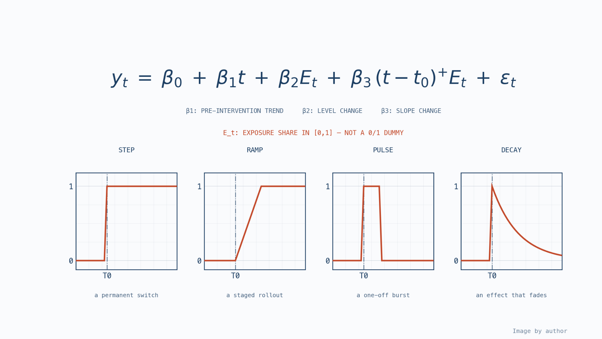
The segmented regression ITSAgentic matches: y_t = β0 + β1·t + β2·E_t + β3·(t − t0)⁺·E_t + ε_t, the place β1 is the pre-intervention pattern, β2 the extent change and β3 the slope change. E_t is an publicity share between 0 and 1, not a 0/1 dummy. 4 panels present the shapes it could take: a step (a everlasting change), a ramp (a staged rollout), a pulse (a one-off burst) and a decay (an impact that fades).

So the intervention enters the regression as an publicity share E_t between 0 and 1 as a substitute of a change. Technically it is one vector, constructed from the intervention date and the form you declare:

• Step is the basic indicator, 1 from T0 onward.

• Ramp interpolates linearly from 0 to 1 throughout the rollout window and holds at 1 afterwards.

• Pulse is 1 in the course of the burst and 0 on both facet.

• Decay follows $e^{-(t – t_0)/tau}$

Coefficients are now not learn as a uncooked degree and slope change, however as degree and slope change per unit of publicity.

What this buys is precision you have been already entitled to. Take the staged market rollout: in the event you code it as a step on the primary launch date, you are telling the mannequin that the entire viewers was handled from day one, when most of it wasn’t. These early post-intervention days are largely untreated customers, they usually pull the estimate towards zero: an actual impact will get diluted into “no important change”. The standard escape is to maneuver T0 to the day the rollout accomplished and discard the weeks in between, which swaps one bias for the lack of half your post-intervention knowledge. With an publicity share you do not have to decide on: daily enters the mannequin weighted by how a lot of the viewers had truly been reached by then.

And the deeper level is that the depth of the therapy is one thing you already know. the site visitors allocation, you realize the launch calendar, you realize the day the marketing campaign was switched off. That data sits in a ticket or a spreadsheet, and a standard pre/publish comparability throws it away. Encoding it in E_t prices no additional knowledge: it simply stops you from discarding what you may have.

One assumption rides together with this: the mannequin treats impact as linear in publicity, so 40% of the viewers reached is assumed to supply 40% of the impact. If the customers reached first reply otherwise from those reached final (attributable to novelty results, for instance), E_t is carrying two issues directly, depth and composition, and the coefficient cannot inform them aside.

Encoding diagnostic checks for the principle assumptions

The assumptions should maintain earlier than and in the course of the evaluation, however how can we make sure that the agent truly checks the assumptions we listed firstly of this publish? For those who assume immediate engineering is an efficient selection, that is for you.

More often than not your agent will ignore the assumptions. A immediate is generally a wishlist however what you want is a guidelines. So ITSAgentic computes the form of the issue deterministically, in plain Python, earlier than the agent will get to purpose about something. These are actual traces from the case that opened this text:

> load_datastanding                okaydate_range            2024-03-01 → 2026-03-01observations          731 (694 pre, 37 publish)raw_diff_pct          +15.29%pre_trend_rsq         0.2209pre_trend_slope_pval  <0.001pre_end_excursion_z   0.98pre_both_halves_sig   true

Take a look at two issues in that output. This can be a completely different collection from the one in Determine 1 however raw_diff_pct: 15.29 is identical species of quantity: the naive pre/publish comparability, the one which will get introduced in a gathering as “+15% since launch”. Right here it is simply one other deterministic discipline, computed and on the report earlier than anybody will get enthusiastic about it. And proper under it, three values describing the form of the pre-intervention interval.

• pre_trend_rsq: was the collection already trending earlier than the intervention?

• pre_end_excursion_z: to measure what occurred proper earlier than the intervention: was it something regular or not?

• pre_both_halves_sig: is the pattern regular throughout the entire pre-period, or pushed by one stretch of it?

Word the worth it truly returned: pre_trend_rsq: 0.22. There’s a pre-existing pattern right here (pre_trend_slope_pval: 0.001), nevertheless it explains solely a fifth of the variance. That’s precisely the form of factor you need measured fairly than eyeballed, and it is the quantity that may resolve, two steps later, how a lot weight the extrapolated counterfactual can carry.

> check_stationarityADF   p = 0.1576    non-stationaryKPSS  p = 0.1000    stationaryBattle detected:ADF and KPSS disagree → attainable weak unit rootRouting resolution:   NON-STATIONARY

Then the textbook checks run, they usually disagree. The ADF check fails to reject a unit root (p-value = 0.16), whereas KPSS fails to reject stationarity. Taken collectively, that is inconclusive fairly than a clear statistical verdict. As an alternative of asking the LLM to resolve the paradox, the device applies a hard and fast conservative routing rule, treating the collection as non-stationary for mannequin choice whereas recording each outcomes and the battle. The routing resolution is repeatable, despite the fact that the statistical proof stays ambiguous.

> check_autocorrelationDurbin–Watson       1.296Ljung–Field lag 1     p < 0.001Ljung–Field lag 7     p < 0.001Ljung–Field lag 14    p < 0.001Ljung–Field lag 30    p < 0.001Autocorrelation:    TRUERouting resolution:   HAC customary errors

And the autocorrelation assumption is just not a warning in a immediate both. Durbin-Watson at 1.30, Ljung-Field important at each lag: has_autocorrelation: TRUE. Downstream, that single flag is what forces the estimator selection towards HAC customary errors.

Every of those three values speaks to one of many assumptions above:

• pre_trend_rsq guards the massive one, counterfactual continuity: in a single-group design the counterfactual is the extrapolated pre-trend.

• pre_end_excursion_z guards no-anticipation: an irregular baseline proper earlier than T0 means the world moved earlier than you probably did.

• pre_both_halves_sig guards towards studying a neighborhood stretch as a world pattern: it checks whether or not the slope holds in each halves of the pre-period, in the identical route.

The important thing level of all of this part is that it is best to compute diagnostics tied to the assumptions of your evaluation and never delegate them to a stochastic output from an LLM. We use the LLM for reasoning functions: we wish the LLM to freely use the instruments however their outputs should all the time be the identical to ensure there is not any essential deviation from the suggestions of the agent.

Are the outcomes and suggestions reliable?

In March 2026 Andrej Karpathy launched Autoresearch and we have been simply looking for the very best answer to enhance ITSAgentic by analysis with completely different datasets. We tailored that loop to ITSAgentic: modify one element, rerun the total benchmark, measure, preserve or revert.

We used greater than 150 completely different datasets (actual, semi-synthetic and artificial instances) and in contrast each run towards a floor fact: for every state of affairs, the injected impact, whether or not detection is predicted, its route, and the warnings the agent should increase.

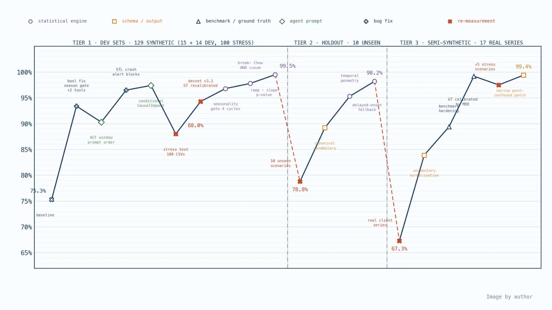
Each iteration of the analysis loop, scored towards floor fact throughout three tiers of datasets. Tier 1, 129 artificial improvement units, climbs from a 75.3% baseline to 99.5%, with a dip to 88.0% when 100 stress-test CSVs are added. Tier 2, 10 unseen holdout situations, drops to 78.8% and recovers to 98.2%. Tier 3, 17 semi-synthetic collection constructed on actual knowledge, drops to 67.3% and recovers to 99.4%. Marker shapes present what modified at every step: statistical engine, output schema, benchmark and floor fact, agent immediate, bug repair or re-measurement.

Each level on that line is one iteration of the loop: edit one thing, run the total benchmark, measure, preserve or discard. The marker color tells you what was edited: the statistical engine, the output schema, the agent’s immediate, the benchmark itself, or a plain bug. The peak is the mixed rating towards the bottom fact. The three bands are three separate periods with datasets of a unique nature. That determine is the experiment log itself, not one thing I drew afterwards to elucidate it.

A phrase on what that rating means, as a result of every little thing on this part hangs on it. Every run is evaluated by two layers: deterministic checks account for 40% of the rating, whereas an LLM choose accounts for the remaining 60%. The deterministic layer checks the output towards the bottom fact: did it detect an impact when detection was anticipated (and keep away from claiming detection when it was not) did it get the route proper, was the estimated magnitude inside ±30% of the true impact, did it classify stationarity accurately, did it keep away from an inappropriate check, and the way lots of the state of affairs’s planted traps did it increase as warnings?

The LLM choose scores 5 dimensions of the written output: diagnostic high quality, mannequin choice, interpretation, honesty about caveats, and enterprise communication. It carries extra weight as a result of ITSAgentic is just not solely anticipated to calculate the best end result, but additionally to purpose about it and talk it effectively sufficient to help a enterprise resolution.

I do know the drops get your consideration however the level is what sort of repair drives every restoration. Tier 1 climbs on bug fixes and statistical work: a boolean serialised unsuitable, a seasonality gate, a structural-break rule. Tier 2 climbs on the temporal-geometry overrides however Tier 3 is completely different: not one change to the statistical engine, not one to the immediate.

The recoveries got here from two sorts of semantic work. Most of it was alignment: normalising the output vocabulary in order that what the agent stated matched what the evaluator anticipated to listen to: the reply was proper, the phrases have been unsuitable. And twice, it was the examination itself: one state of affairs demanded detection of a +5% impact that sits under the minimal detectable impact for that collection; one other demanded a optimistic verdict on an impact with p-value=0.996 when you extrapolate the pre-trend.

In each instances the agent returned “detected: false” with low confidence (and that was the right inference) as a result of an impact {that a} collection lacks the ability to detect is just not an impact you possibly can report. Word the excellence, as a result of the bottom fact did not make it both: the +5% was actually injected. What was unsuitable wasn’t the reality, it was the examination grading a real impact as if it have been a detectable one.

Which is the true discovering? Iteration by iteration, the enhancements confirmed up. The arithmetic issues got here first, then the statistical ones, and the final stretch was all semantics. By the point the system met actual knowledge, its statistical core did not want one other line of code.

What ITSAgentic cannot repair however why I like to recommend it

Let me be trustworthy about the place this technique stands. ITSA is a implausible device: it takes your evaluation one actual step past evaluating averages however it’s not, by a protracted shot, the strongest identification technique within the quasi-experimental toolbox.

In my view, it has two structural issues. The primary is that the entire design leans on the pre-trend having sufficient predictive power to be the counterfactual: as Morgan and Winship present, when the true counterfactual bends the linear extrapolation would not fail loudly, it quietly overestimates the impact on each single post-intervention day.

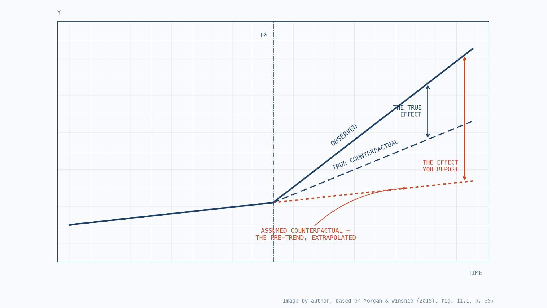
Why a linear counterfactual can mislead. Earlier than the intervention the collection follows a mild pattern. After T0, noticed values rise steeply, however the true counterfactual, what would have occurred anyway, additionally bends upward. Interrupted Time Collection Evaluation assumes the pre-trend merely continues, so the assumed counterfactual is flatter. The hole you report is far bigger than the true impact, and it overestimates the impact on each post-intervention day. Primarily based on Morgan & Winship (2015), fig. 11.1, p. 357.

The second downside is the mirror picture: the design attributes to the intervention any deviation from the projected trajectory, whether or not the intervention brought about it or not. Linden factors to the foundation of the issue: a single-group ITSA has no management group, so the projected pre-intervention trajectory should play that function. Covariates can modify for noticed time-varying confounders and enhance the counterfactual prediction, however they can’t rule out unobserved shocks that coincide with the intervention. This is the reason difference-in-differences or artificial management may be extra defensible when a reputable comparability collection is obtainable.

These are the boundaries of the tactic however ITSAgentic has one among its personal: there is a household of checks it would not run but. The primary is the in-time placebo: re-run the evaluation with a faux intervention date someplace within the pre-period, the place nothing occurred. If the pipeline experiences an impact there, the design is leaking and that one check says extra about whether or not you possibly can belief a end result than any diagnostic on this article.

The second is sensitivity: how a lot does the estimate transfer if T0 shifts by a couple of days, or if the declared publicity form is unsuitable? The form and half-life are declared as soon as, earlier than the evaluation, and recorded, which is the minimal defence towards tuning the geometry till the p-value cooperates. However declaring a parameter is not the identical as figuring out how a lot the reply leans on it.

And but that is precisely the tactic price turning into an AI product. Counterfactual reasoning has lived for years behind a wall of specialized knowledge scientists. Somebody in advertising and marketing or product can now add a CSV, declare an intervention date, and get again an evaluation with a counterfactual, uncertainty, and warnings that till lately required a specialist who most corporations haven’t got.

That is the Computer virus. ITSA makes counterfactuals explainable: one line for what occurred, one line for what would have occurred, and the impact is the hole. A non-technical stakeholder will get that. As soon as your group thinks in counterfactuals, you have earned the credibility to usher in the extra complicated (and better-identified) designs. We won’t overlook there’s enterprise in every little thing we do and stakeholder administration is a part of it.

Generative AI places knowledge merchandise like this one inside attain in a method that wasn’t true two years in the past, however pay attention to this: the output needs to be protected and prescribed, and meaning deterministic instruments and closed parameters that assure the identical enter all the time produces the identical numbers, whereas the mannequin’s reasoning is spent the place it truly pays, on deciding what to run and what the end result means (and anticipating in all probability barely completely different interpretations on the identical knowledge). That is the entire structure of this text in a single sentence, and it is the half I would preserve even when every little thing else modified.

Sources:

1. Linden, A. (2015). Conducting interrupted time-series evaluation for single- and multiple-group comparisons. The Stata Journal, 15(2), 480–500. — SAGE · PDF

2. Linden, A. (2017). Challenges to validity in single-group interrupted time collection evaluation. Journal of Analysis in Medical Observe, 23(2). — Wiley

3. Linden, A. (2016). Persistent threats to validity in single-group interrupted time collection evaluation with a crossover design. — PubMed

4. Morgan, S. L., & Winship, C. (2015). Counterfactuals and causal inference: Strategies and rules for social analysis (2nd ed.). Cambridge College Press.

5. Karpathy, A. (2026). autoresearch — github.com/karpathy/autoresearch.

6. Brodersen, Okay. H., et al. (2015). Inferring causal affect utilizing Bayesian structural time-series fashions. Annals of Utilized Statistics, 9(1), 247–274.

7. Lopez Bernal, J., Cummins, S., & Gasparrini, A. (2017). Interrupted time collection regression for the analysis of public well being interventions: A tutorial. Worldwide Journal of Epidemiology, 46(1), 348–355.