How Far Can Classical NLP Go? From Bag-of-Phrases to Stacking on Spooky Writer Identification

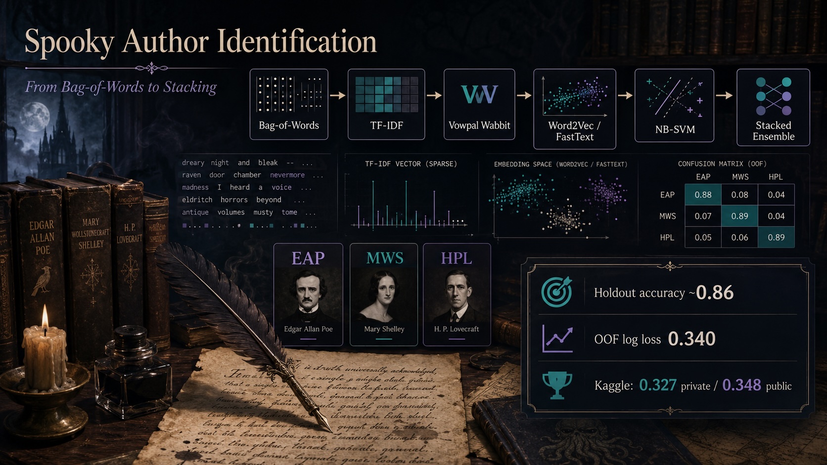
is an efficient method to take a look at NLP fashions as a result of it focuses not solely on what a sentence says, but additionally on how it’s written. Kaggle’s Spooky Writer Identification competitors is a compact model of this problem: given a single sentence from gothic or horror fiction, the mannequin has to foretell whether or not it was written by Edgar Allan Poe (EAP), Mary Wollstonecraft Shelley (MWS), or H. P. Lovecraft (HPL).

At first, this looks as if a typical three-class textual content classification downside. However in actuality, it’s extra complicated. The authors all write about comparable themes: concern, thriller, loss of life, environment, and the supernatural. Easy key phrases usually are not sufficient to inform them aside. As a substitute, the essential clues are sometimes stylistic: perform phrases, punctuation, character patterns, quick phrases, sentence rhythm, and the best way every writer builds a sentence.

This made the mission a great way to discover a selected query:

How far can classical NLP go once we select representations fastidiously and consider them actually?

I approached the duty by constructing a sequence of more and more succesful classical fashions:

1. a quick Vowpal Wabbit phrase baseline,
2. a richer VW mannequin with punctuation and character n-grams,
3. a tuned TF-IDF ensemble,
4. a stacked sparse-text ensemble utilizing out-of-fold predictions,
5. a small illustration survey evaluating sparse options, BM25, Word2Vec, and FastText.

The aim was not solely to enhance the rating, but additionally to grasp which representations helped, which metrics improved, and which analysis setup every consequence got here from.

This text focuses on the mission’s methodology, outcomes, and interpretation. I’ll go over the principle implementation selections and share the important thing code snippets, however I received’t embody each line from the pocket book. The entire executed pocket book, together with the total implementation and outputs, is on the market within the GitHub repository linked on the finish.

Dataset and Analysis Setup

The dataset accommodates 19,579 labeled coaching sentences and 8,392 unlabeled take a look at sentences. The category distribution is mildly imbalanced:

I encoded the labels as 1-based integers as a result of Vowpal Wabbit’s One-In opposition to-All multiclass mode expects labels beginning at 1.

train_texts = pd.read_csv(DATA_DIR / "practice.csv", index_col="id")
test_texts = pd.read_csv(DATA_DIR / "take a look at.csv", index_col="id")

AUTHOR_CODE = {"EAP": 1, "MWS": 2, "HPL": 3}
train_texts["author_code"] = train_texts["author"].map(AUTHOR_CODE)

print(f"Practice: {len(train_texts)} sentences   Check: {len(test_texts)} sentences")
print(train_texts["author"].value_counts(normalize=True).spherical(3))

To match fashions regionally, I used a single stratified 70/30 train-validation cut up with a set random seed. This stored the category proportions steady and ensured that each mannequin was evaluated on the identical held-out examples.

train_texts_part, valid_texts = train_test_split(
    train_texts,
    test_size=0.3,
    random_state=17,
    stratify=train_texts["author_code"]
)

y_part = train_texts_part["author_code"].values
y_valid = valid_texts["author_code"].values

I centered on three foremost metrics:

• Accuracy: easy to grasp, but it surely solely measures the ultimate top-class resolution.
• Macro-F1: helpful for checking whether or not efficiency is balanced throughout the three authors.
• Multiclass log loss: the official Kaggle metric and a very powerful metric for this mission, as a result of it evaluates the standard of the anticipated possibilities, not simply the anticipated class.

Log loss rewards assured appropriate predictions and closely penalizes assured unsuitable predictions. This issues in a contest the place the submission is a chance distribution over EAP, HPL, and MWS.

1. Phrase-only Vowpal Wabbit baseline

I began with Vowpal Wabbit as a result of it’s quick, handles sparse information properly, and is well-suited to linear textual content fashions. VW trains on-line linear fashions, hashes options into a set function area, and handles multiclass classification via One-In opposition to-All.

For the primary baseline, I used solely lowercased phrase options of size three or extra.

def to_vw_words(df, is_train=True):
    """VW line: ' |textual content '."""
    traces = []

    for i in vary(len(df)):
        label = df["author_code"].iloc[i] if is_train else 1
        textual content = df["text"].iloc[i].decrease().substitute("|", "").substitute(":", "")
        phrases = " ".be a part of(re.findall(r"w{3,}", textual content))
        traces.append(f"{label} |textual content {phrases}n")

    return traces

One implementation element that mattered was how VW handles a number of passes. When VW reads a file straight, choices reminiscent of passes and cache behave as anticipated. When feeding examples manually via the Python API, I needed to loop over the file myself.

N_PASSES = 10

vw = Workspace(
    oaa=3,
    loss_function="logistic",
    ngram=2,
    b=28,
    quiet=True,
    final_regressor=f"{OUTPUT_DIR}/spooky_words.vw"
)

for _ in vary(N_PASSES):
    with open(f"{OUTPUT_DIR}/train_words.vw") as f:
        for line in f:
            vw.be taught(line)

vw.end()

On the 70/30 holdout cut up, the word-only VW baseline reached:

This was already a robust consequence for a quick linear mannequin utilizing easy phrase and bigram options. It additionally established a helpful baseline: any added illustration or ensemble layer wanted to clear this bar.

2. Wealthy VW: including style-aware options

Authorship attribution includes greater than classifying subjects. A mannequin additionally wants entry to cues that replicate writing type. For the richer VW mannequin, I separated the enter into three namespaces:

• |w for phrases, together with quick perform phrases,
• |p for punctuation,
• |c for character n-grams.

def char_ngrams(textual content, ns=(2, 3, 4)):
    """Boundary-aware character n-grams; whitespace/edges develop into '_'."""
    t = "_" + re.sub(r"s+", "_", textual content.strip()) + "_"
    return [t[i:i + n] for n in ns for i in vary(len(t) - n + 1)]


def to_vw_rich(df, is_train=True, char_ns=(2, 3, 4)):
    """Three namespaces: |w phrases, |p punctuation, |c character n-grams."""
    traces = []
    texts = df["text"].values
    labels = df["author_code"].values if is_train else None

    for i, textual content in enumerate(texts):
        secure = str(textual content).decrease().substitute("|", " ").substitute(":", " ")

        label = labels[i] if is_train else 1
        phrases = " ".be a part of(re.findall(r"w+", secure))
        punct = " ".be a part of(re.findall(r"[^ws]", secure))
        chars = " ".be a part of(char_ngrams(secure, ns=char_ns))

        traces.append(f"{label} |w {phrases} |p {punct} |c {chars}n")

    return traces

This mannequin used extra passes and a barely bigger hash area than the word-only baseline.

N_PASSES = 15

vw = Workspace(
    oaa=3,
    loss_function="logistic",
    ngram=2,
    b=29,
    quiet=True,
    final_regressor=f"{OUTPUT_DIR}/spooky_rich.vw"
)

for _ in vary(N_PASSES):
    with open(f"{OUTPUT_DIR}/train_rich.vw") as f:
        for line in f:
            vw.be taught(line)

vw.end()

This improved the holdout consequence:

The acquire is significant: including punctuation and character-level construction helped the mannequin seize type past plain phrase selection.

3. TF-IDF phrase and character options

Subsequent, I wished to see whether or not one other classical sparse-text pipeline might match or exceed the VW outcomes. I constructed a TF-IDF function matrix utilizing two views of the textual content:

1. word-level unigrams and bigrams,
2. character-level 2-to-5-grams inside phrase boundaries.

CLASSES = np.array([1, 2, 3])  # 1=EAP, 2=MWS, 3=HPL

def build_tfidf(fit_texts):
    word_vectorizer = TfidfVectorizer(
        sublinear_tf=True,
        ngram_range=(1, 2),
        min_df=2
    ).match(fit_texts)

    char_vectorizer = TfidfVectorizer(
        sublinear_tf=True,
        analyzer="char_wb",
        ngram_range=(2, 5),
        min_df=2
    ).match(fit_texts)

    return word_vectorizer, char_vectorizer


def tfidf_features(word_vectorizer, char_vectorizer, texts):
    X_word = word_vectorizer.remodel(texts)
    X_char = char_vectorizer.remodel(texts)
    return sp.hstack([X_word, X_char]).tocsr()

The phrase options seize vocabulary and phrase-level proof. The character options seize spelling fragments, suffixes, prefixes, punctuation-adjacent patterns, and different small particulars which might be helpful for type classification.

I educated three complementary fashions on this illustration:

• Logistic Regression,
• NB-SVM-style Logistic Regression,
• Complement Naive Bayes.

For Logistic Regression and the NB-SVM-style mannequin, I tuned the C values with inside cross-validation on the coaching cut up solely, leaving the holdout set untouched.

def tune_lr_C(X, y, C_grid=(0.1, 0.3, 1, 3, 10, 30), n_splits=5):
    cv = StratifiedKFold(n_splits=n_splits, shuffle=True, random_state=42)
    rows = []

    for C in C_grid:
        oof = np.zeros((X.form[0], len(CLASSES)))

        for tr_idx, va_idx in cv.cut up(X, y):
            clf = LogisticRegression(C=C, max_iter=3000)
            clf.match(X[tr_idx], y[tr_idx])
            oof[va_idx] = align_proba(clf, X[va_idx])

        rows.append({"C": C, "log_loss": log_loss(y, oof, labels=CLASSES)})

    return pd.DataFrame(rows)

One of the best inner-CV tuning outcomes have been:

The ultimate 3-model chance common reached:

The accuracy acquire over wealthy VW was modest, however the log loss was robust. Since Kaggle evaluates chance distributions, this was an essential enchancment.

NB-SVM-style Logistic Regression

The NB-SVM-style mannequin will get its personal part as a result of it’s a easy but efficient classical text-classification trick.

The thought is to compute a per-feature log-count ratio: how far more usually a function seems in a single class than within the others. Every function is then multiplied by this ratio earlier than becoming a linear classifier.

def nbsvm_proba(X_train, y_train, X_test, C=10):
    probas = []

    for cls in CLASSES:
        y_binary = (y_train == cls).astype(int)

        p = X_train[y_binary == 1].sum(axis=0) + 1
        q = X_train[y_binary == 0].sum(axis=0) + 1

        r = np.log((p / p.sum()) / (q / q.sum()))
        r = np.asarray(r).ravel()

        clf = LogisticRegression(C=C, max_iter=3000)
        clf.match(X_train.multiply(r), y_binary)

        probas.append(clf.predict_proba(X_test.multiply(r))[:, 1])

    proba = np.vstack(probas).T
    proba = np.clip(proba, 1e-15, 1 - 1e-15)
    return proba / proba.sum(axis=1, keepdims=True)

Regardless of the title, my implementation shouldn’t be a pure SVM. It makes use of Logistic Regression educated on Naive-Bayes-weighted sparse options. The profit is that options strongly related to a selected writer are amplified earlier than the linear mannequin is educated.

4. Stacking with out-of-fold predictions

After the TF-IDF ensemble, I had a number of helpful base fashions. A flat common provides every mannequin equal weight, however there is no such thing as a cause to imagine each mannequin is equally dependable for each class. Stacking lets a second-level mannequin learn to mix them.

The primary leakage threat is coaching the meta-learner on predictions from base fashions which have already seen the identical examples. To keep away from that, I used out-of-fold predictions:

• For coaching examples, every base mannequin predicts solely the examples in a fold that it was not educated on.
• For holdout or take a look at examples, predictions are averaged throughout fold-trained variations of every base mannequin.

The bottom fashions have been:

BASE_MODELS = ["lr", "nbsvm", "cnb", "mnb", "sgd"]

BASE_PARAM_GRIDS = {
    "lr": {"C": [1, 3, 10, 30]},
    "nbsvm": {"C": [1, 3, 10, 30]},
    "cnb": {"alpha": [0.1, 0.3, 0.5, 1.0]},
    "mnb": {"alpha": [0.1, 0.3, 0.5, 1.0]},
    "sgd": {"alpha": [1e-6, 3e-6, 1e-5, 3e-5]},
}

The stacking function builder creates a matrix with one block of chance columns per base mannequin. With 5 base fashions and three authors, the meta-learner receives 15 chance options per instance.

def build_stack_features(X_train, y_train, X_test, best_params_by_model,
                         n_folds=5, seed=17):
    skf = StratifiedKFold(n_splits=n_folds, shuffle=True, random_state=seed)

    n_classes = len(CLASSES)
    n_models = len(BASE_MODELS)

    oof_stack = np.zeros((X_train.form[0], n_classes * n_models))
    test_stack = np.zeros((X_test.form[0], n_classes * n_models))

    for j, type in enumerate(BASE_MODELS):
        begin = j * n_classes
        finish = begin + n_classes
        params = best_params_by_model[kind]

        for tr_idx, va_idx in skf.cut up(X_train, y_train):
            oof_stack[va_idx, start:end] = base_proba(
                type,
                X_train[tr_idx],
                y_train[tr_idx],
                X_train[va_idx],
                params
            )

            test_stack[:, start:end] += base_proba(
                type,
                X_train[tr_idx],
                y_train[tr_idx],
                X_test,
                params
            ) / n_folds

    return oof_stack, test_stack

I tuned the Logistic Regression meta-learner utilizing cross-validation on the stacked chance options.

def tune_meta_C(oof_stack, y, C_grid=(0.03, 0.1, 0.3, 1, 3, 10, 30)):
    skf = StratifiedKFold(n_splits=5, shuffle=True, random_state=17)

    for C in C_grid:
        oof_meta = np.zeros((oof_stack.form[0], len(CLASSES)))

        for tr_idx, va_idx in skf.cut up(oof_stack, y):
            meta = LogisticRegression(C=C, max_iter=3000)
            meta.match(oof_stack[tr_idx], y[tr_idx])
            oof_meta[va_idx] = align_proba(meta, oof_stack[va_idx])

        print(C, log_loss(y, oof_meta, labels=CLASSES))

On the 70/30 holdout cut up, one of the best base-model settings have been:

One of the best meta-learner setting was C=3.

The stacked mannequin reached:

This was the strongest holdout consequence within the mission. The most important enchancment was not uncooked accuracy; it was log loss. Which means the ensemble improved the chance estimates, which is strictly what the Kaggle metric rewards.

5. Last full-data refit and Kaggle submission

For the ultimate submission, I refit the TF-IDF illustration on the total labeled coaching information, rebuilt the stacking options, retuned the bottom fashions, educated the ultimate meta-learner, and generated predictions for the take a look at set.

On the total coaching information, one of the best base-model parameters have been:

One of the best remaining meta-learner setting was C=30.

The code additionally explicitly mapped my inner class order [1, 2, 3] = [EAP, MWS, HPL] into Kaggle’s required submission column order: EAP, HPL, MWS.

meta_final = LogisticRegression(C=best_full_meta_C, max_iter=3000)
meta_final.match(oof_full, y_full)

proba_test = align_proba(meta_final, test_stack)

proba_test = np.clip(proba_test, 1e-15, 1 - 1e-15)
proba_test = proba_test / proba_test.sum(axis=1, keepdims=True)

submission = pd.DataFrame({
    "id": test_texts.index,
    "EAP": proba_test[:, 0],   # class 1
    "HPL": proba_test[:, 2],   # class 3
    "MWS": proba_test[:, 1],   # class 2
})

submission.to_csv(OUTPUT_DIR / "spooky_submission.csv", index=False)

The total-data level-2 OOF estimate for the meta-learner was:

This quantity is helpful as a sanity examine, but it surely shouldn’t be in contrast straight with the sooner 70/30 holdout rows as a result of it comes from a special analysis setup. It evaluates the meta-learner utilizing out-of-fold stacking options over the total coaching information, not a totally nested cross-validation of your complete pipeline.

On Kaggle, the ultimate stacked mannequin scored:

The leaderboard scores landed near the full-data level-2 OOF estimate, which is encouraging. I’d nonetheless deal with that as validation proof, not proof that the setup is totally unbiased.

6. Error evaluation

Mixture metrics are helpful, however they will disguise the place the mannequin fails. I used the holdout predictions from the stacked mannequin to examine the confusion matrix, per-author recall, and high-confidence errors.

AUTHORS = {1: "EAP", 2: "MWS", 3: "HPL"}

cm = confusion_matrix(y_valid, valid_predictions, labels=CLASSES)

cm_df = pd.DataFrame(
    cm,
    index=[f"true_{AUTHORS[c]}" for c in CLASSES],
    columns=[f"pred_{AUTHORS[c]}" for c in CLASSES]
)

show(cm_df)

The confusion matrix was:

Per-author recall was comparatively balanced:

The most typical confusions have been:

The primary level is that the mannequin didn’t merely collapse into predicting the biggest class. The recall scores have been shut throughout all three authors, and the errors have been bidirectional. MWS and EAP have been usually confused with one another, whereas HPL and EAP additionally overlapped on some quick or stylistically impartial sentences.

I additionally inspected high-confidence errors. One instance was the sentence:

“I walked the cellar from finish to finish.”

The true writer was EAP, however the mannequin assigned HPL a chance above 0.97. This can be a helpful reminder that single-sentence authorship will be underdetermined. Some sentences merely don’t carry sufficient distinctive stylistic proof for a sparse linear mannequin to separate three comparable gothic authors reliably.

7. A illustration survey

To place the principle pipeline in context, I additionally examined a number of foundational representations on the identical holdout cut up.

For Bag-of-Phrases, I used phrase counts with unigrams and bigrams:

bow = CountVectorizer(
    ngram_range=(1, 2),
    min_df=2
)

X_bow_tr = bow.fit_transform(train_texts_part["text"])
X_bow_va = bow.remodel(valid_texts["text"])

bow_lr = LogisticRegression(C=10, max_iter=3000)
bow_lr.match(X_bow_tr, y_part)

For BM25, I handled retrieval as a nearest-neighbor classifier. This isn’t BM25’s pure use case, but it surely was helpful as a degree of comparability.

Ok = 15
scores = np.asarray((query_terms[start:end] @ bm25_docs.T).todense())
topk = np.argpartition(-scores, kth=Ok - 1, axis=1)[:, :K]

For Word2Vec and FastText, I educated embeddings on the coaching cut up, then represented every sentence as an IDF-weighted common of its phrase vectors.

def document_vectors(mannequin, tokenized_docs):
    vectors = np.zeros((len(tokenized_docs), mannequin.vector_size), dtype=np.float32)

    for i, tokens in enumerate(tokenized_docs):
        doc_vecs, doc_weights = [], []

        for token in tokens:
            attempt:
                doc_vecs.append(mannequin.wv[token])
                doc_weights.append(idf_weight.get(token, 1.0))
            besides KeyError:
                proceed

        if doc_vecs:
            vectors[i] = np.common(doc_vecs, axis=0, weights=doc_weights)

    return vectors

The outcomes have been:

Sparse count-based options have been clearly stronger on this setup than easy averaged embeddings. That doesn’t imply Word2Vec or FastText are usually weak. It signifies that for this short-text authorship job, averaging phrase vectors blurred most of the stylistic particulars that sparse phrase, character, and punctuation options preserved.

Outcomes at a look

All holdout rows use the identical stratified 70/30 cut up, so they’re straight comparable.

Kaggle submission:

The extent-2 OOF estimate shouldn’t be straight similar to the holdout rows as a result of it makes use of a special analysis setup.

What really helped

Many of the helpful enhancements got here from higher representations and cleaner validation, not from including complexity for its personal sake.

Sparse phrase and character options carried the strongest sign.
The duty is stylistic, and sparse n-gram options preserved particulars that pooled dense vectors tended to clean away.

Punctuation and character n-grams improved authorship modeling.
Including style-aware options elevated the VW holdout accuracy from 0.8332 to 0.8553.

TF-IDF improved chance high quality.
The tuned TF-IDF ensemble didn’t dramatically enhance accuracy, but it surely produced a robust log loss consequence, which is what the competitors optimizes.

Stacking helped most with log loss.
The stacked mannequin improved holdout log loss from 0.3843 to 0.3504. This means that the meta-learner discovered a greater method to mix chance estimates than a flat common.

Analysis separation issues.
I stored three consequence varieties separate: the 70/30 holdout, the full-data level-2 OOF estimate, and the Kaggle leaderboard scores. They reply totally different questions, so mixing them would make the outcomes look extra sure than they are surely.

Limitations and subsequent steps

There are a number of methods I’d lengthen this mission.

First, the stacking pipeline was evaluated with a single holdout cut up plus a full-data level-2 OOF estimate. A totally nested cross-validation design would supply a extra conservative estimate of the entire modeling and tuning course of.

Second, I used log loss as the principle probability-quality metric, however I didn’t embody specific calibration diagnostics reminiscent of reliability diagrams or anticipated calibration error. For the reason that remaining goal is chance high quality, calibration evaluation can be a pure subsequent step.

Third, I didn’t examine towards a transformer baseline reminiscent of DistilBERT or BERT. A fine-tuned transformer can be the plain subsequent benchmark, particularly to check how a lot contextual illustration improves over sparse classical options on quick literary sentences.

Fourth, the hyperparameter search was deliberately restricted. A broader search over TF-IDF ranges, VW settings, smoothing values, regularization strengths, and stacking design selections might enhance the ultimate rating.

Lastly, the dataset is small and domain-specific. These outcomes help conclusions about short-text authorship attribution on this setting, not a common rating of NLP strategies.

Conclusion

This mission reveals that classical NLP can nonetheless go surprisingly far when the illustration matches the issue. A word-only Vowpal Wabbit baseline was already robust, however including style-aware options, TF-IDF phrase and character n-grams, probability-focused tuning, and stacked generalization additional improved the mannequin.

The strongest classical pipeline reached 0.8687 accuracy and 0.3504 log loss on the 70/30 holdout cut up, and the ultimate stacked submission scored 0.30414 non-public and 0.33621 public log loss on Kaggle.

The primary takeaway is not only that stacking improved the rating. It’s that authorship attribution rewards the small print: punctuation, subword patterns, perform phrases, and cautious chance estimates. Earlier than reaching for heavier contextual fashions, a well-validated sparse-text baseline can nonetheless be a severe competitor.

Knowledge supply and license

This text makes use of Kaggle’s Spooky Writer Identification dataset, a text-classification dataset constructed from excerpts of public-domain fiction by Edgar Allan Poe, H. P. Lovecraft, and Mary Wollstonecraft Shelley. The duty is to foretell the writer of every sentence amongst three labels: EAP for Edgar Allan Poe, HPL for H. P. Lovecraft, and MWS for Mary Wollstonecraft Shelley.

The dataset is listed on Kaggle below the CC BY 4.0 license. This license permits sharing and adaptation, together with for business functions, offered acceptable attribution is given. On this article, the dataset is used for an academic machine-learning walkthrough, and attribution hyperlinks are offered on this part.

Thanks for making all of it the best way to the tip! I hope you discovered this mission as enjoyable and helpful as I did. In case you have ideas, questions, or concepts for extending the experiment, be happy to succeed in out via LinkedIn or my web site.

Hyperlinks

• Full pocket book + code
• LinkedIn
• Web site