


On this article, I’ll introduce you to hierarchical Bayesian (HB) modelling, a versatile strategy to mechanically mix the outcomes of a number of sub-models. This methodology allows estimation of individual-level results by optimally combining info throughout completely different groupings of knowledge by means of Bayesian updating. That is notably precious when particular person models have restricted observations however share widespread traits/behaviors with different models.
The next sections will introduce the idea, implementation, and various use circumstances for this methodology.
The Drawback with Conventional Approaches
As an software, think about that we’re a big grocery retailer making an attempt to maximise product-level income by setting costs. We would wish to estimate the demand curve (elasticity) for every product, then optimize some revenue maximization perform. As step one to this workstream, we would wish to estimate the value elasticity of demand (how responsive demand is to a 1% change in worth) given some longitudinal information with $i in N$ merchandise over $t in T$ intervals. Do not forget that the value elasticity of demand is outlined as:
$$beta=frac{partial log{textrm{Items}}_{it}}{partial log textrm{Value}_{it}}$$
Assuming no confounders, we are able to use a log-linear fixed-effect regression mannequin to estimate our parameter of curiosity:
$$log(textrm{Items}_{it})= beta log(textrm{Value})_{it} +gamma_{c(i),t}+ delta_i+ epsilon_{it}$$
$gamma_{c(i),t}$ is a set of category-by-time dummy variables to seize the common demand in every category-time interval and $delta_i$ is a set of product dummies to seize the time-invariant demand shifter for every product. This “fixed-effect” formulation is commonplace and customary in lots of regression-based fashions to regulate for unobserved confounders. This (pooled) regression mannequin permits us to get better the common elasticity $beta$ throughout all $N$ models. This is able to imply that the shop might goal a mean worth degree throughout all merchandise of their retailer to maximise the income:
$$underset{textrm{Value}_t}{max} ;;; textrm{Value}_{t}cdotmathbb{E}(textrm{Amount}_{t} | textrm{Value}_{t}, beta)$$
If these models have a pure grouping (product classes), we would be capable of determine the common elasticity of every class by working separate regressions (or interacting the value elasticity with the product class) for every class utilizing solely models from that class. This is able to imply that the shop might goal common costs in every class to maximise category-specific income, such that:
$$underset{textrm{Value}_{c(i),t}}{max} ;;; textrm{Value}_{c(i),t}cdotmathbb{E}(textrm{Amount}_{c(i),t} | textrm{Value}_{c(i),t}, beta_{c(i)})$$
With adequate information, we might even run separate regressions for every particular person product to acquire extra granular elasticities.
Nonetheless, real-world information usually presents challenges: some merchandise have minimal worth variation, quick gross sales histories, or class imbalance throughout classes. Underneath these restrictions, working separate regressions to determine product elasticity would doubtless result in massive commonplace errors and weak identification of $beta$. HB fashions addresses these points by permitting us to acquire granular estimates of the coefficient of curiosity by sharing statistical power each throughout completely different groupings whereas preserving heterogeneity. With the HB formulation, it’s doable to run one single regression (just like the pooled case) whereas nonetheless recovering elasticities on the product degree, permitting for granular optimizations.
Understanding Hierarchical Bayesian Fashions
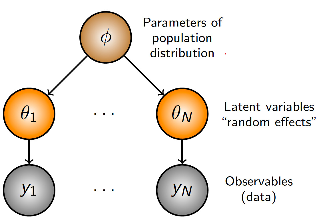
At its core, HB is about recognizing the pure construction in our information. Fairly than treating all observations as fully unbiased (many separate regressions) or forcing them to observe an identical patterns (one pooled regression), we acknowledge that observations can cluster into teams, with merchandise inside every group sharing comparable patterns. The “hierarchical” facet refers to how we arrange our parameters in numerous ranges. In its most simple format, we might have:
- A World parameter that applies to all information.
- Group-level parameters that apply to observations inside that group.
- Particular person-level parameters that apply to every particular particular person.
This technique is versatile sufficient so as to add or take away hierarchies as wanted, relying on the specified degree of pooling. For instance, if we expect there aren’t any similarities throughout classes, we might take away the worldwide parameter. If we expect that these merchandise don’t have any pure groupings, we might take away the group-level parameters. If we solely care concerning the group-level impact, we are able to take away the individual-level parameter and have the group-level coefficients as our most granular parameter. If there exists the presence of subgroups nested inside the teams, we are able to add one other hierarchical layer. The chances are infinite!
The “Bayesian” facet refers to how we replace our beliefs about these parameters based mostly on noticed information. We first begin with a proposed prior distribution that symbolize our preliminary perception of those parameters, then replace them iteratively to get better a posterior distributions that comes with the data from the information. In observe, which means that we use the global-level estimate to tell our group-level estimates, and the group-level parameters to tell the unit-level parameters. Items with a bigger variety of observations are allowed to deviate extra from the group-level means, whereas models with a restricted variety of observations are pulled nearer to the means.
Let’s formalize this with our worth elasticity instance, the place we (ideally) wish to get better the unit-level worth elasticity. We estimate:
$$log(textrm{Items}_{it})= beta_i log(textrm{Value})_{it} +gamma_{c(i),t} + delta_i + epsilon_{it}$$
The place:
- $beta_i sim textrm{Regular}(beta_{cleft(iright)},sigma_i)$
- $beta_{c(i)}sim textrm{Regular}(beta_g,sigma_{c(i)})$
- $beta_gsim textrm{Regular}(mu,sigma)$
The one distinction from the primary equation is that we exchange the worldwide $beta$ time period with product-level betas $beta_i$. We specify that the unit degree elasticity $beta_i$ is drawn from a traditional distribution centered across the category-level elasticity common $beta_{c(i)}$, which is drawn from a shared international elasticity $beta_g$ for all teams. For the unfold of the distribution $sigma$, we are able to assume a hierarchical construction for that too, however on this instance, we simply set primary priors for them to take care of simplicity. For this software, we assume a previous perception of: ${ mu= -2, sigma= 1, sigma_{c(i)}=1, sigma_i=1}$. This formulation of the prior assumes that the worldwide elasticity is elastic, 95% of the elasticities fall between -4 and 0, with a regular deviation of 1 at every hierarchical degree. To check whether or not these priors are accurately specified, we’d do a prior predictive checks (not lined on this article) to see whether or not our prior beliefs can get better the information that we observe.
This hierarchical construction permits info to circulate between merchandise in the identical class and throughout classes. If a selected product has restricted worth variation information, its elasticity can be pulled towards the class elasticity $beta_{c(i)}$. Equally, classes with fewer merchandise can be influenced extra by the worldwide elasticity, which derives its imply from all class elasticities. The great thing about this strategy is that the diploma of “pooling” occurs mechanically based mostly on the information. Merchandise with a number of worth variation will keep estimates nearer to their particular person information patterns, whereas these with sparse information will borrow extra power from their group.
Implementation
On this part, we implement the above mannequin utilizing the Numpyro package deal in Python, a light-weight probabilistic programming language powered by JAX for autograd and JIT compilation to GPU/TPU/CPU. We begin off by producing our artificial information, defining the mannequin, and becoming the mannequin to the information. We shut out with some visualizations of the outcomes.
Information Producing Course of
We simulate gross sales information the place demand follows a log-linear relationship with worth and the product-level elasticity is generated from a Gaussian distribution $beta_i sim textrm{Regular}(-2, 0.7)$. We add in a random worth change each time interval with a $50%$ chance, category-specific time tendencies, and random noise. This provides in multiplicatively to generate our log anticipated demand. From the log anticipated demand, we exponentiate to get the precise demand, and draw realized models bought from a Poisson distribution. We then filter to maintain solely models with greater than 100 models bought (helps accuracy of estimates, not a vital step), and are left with $N=11,798$ merchandise over $T = 156$ intervals (weekly information for 3 years). From this dataset, the true international elasticity is $beta_g = -1.6$, with category-level elasticities starting from $beta_{c(i)} in [-1.68, -1.48]$.
Understand that this DGP ignores quite a lot of real-world intricacies. We don’t mannequin any elements that might collectively have an effect on each costs and demand (akin to promotions), and we don’t mannequin any confounders. This instance is solely meant to point out that we are able to get better the product-specific elasticity beneath a wells-specified mannequin, and doesn’t purpose to cowl methods to accurately determine that worth is exogenous. Nonetheless, I recommend that readers seek advice from Causal Inference for the Courageous and True for an introduction to causal inference.
import numpy as np
import pandas as pd

def generate_price_elasticity_data(N: int = 1000,
                                   C: int = 10,
                                   T: int = 50,
                                   price_change_prob: float = 0.2,
                                   seed = 42) -> pd.DataFrame:
    """
    Generate artificial information for worth elasticity of demand evaluation.
    Information is generated by
    """
    if seed is just not None:
        np.random.seed(seed)

    # Class demand and tendencies
    category_base_demand = np.random.uniform(1000, 10000, C)
    category_time_trends = np.random.uniform(0, 0.01, C)
    category_volatility = np.random.uniform(0.01, 0.05, C)  # Random volatility for every class
    category_demand_paths = np.zeros((C, T))
    category_demand_paths[:, 0] = 1.0
    shocks = np.random.regular(0, 1, (C, T-1)) * category_volatility[:, np.newaxis]
    tendencies = category_time_trends[:, np.newaxis] * np.ones((C, T-1))
    cumulative_effects = np.cumsum(tendencies + shocks, axis=1)
    category_demand_paths[:, 1:] = category_demand_paths[:, 0:1] + cumulative_effects

    # product results
    product_categories = np.random.randint(0, C, N)
    product_a = np.random.regular(-2, .7, dimension=N)
    product_a = np.clip(product_a, -5, -.1)

    # Preliminary costs for every product
    initial_prices = np.random.uniform(100, 1000, N)
    costs = np.zeros((N, T))
    costs[:, 0] = initial_prices

    # Generate random values and whether or not costs modified
    random_values = np.random.rand(N, T-1)
    change_mask = random_values < price_change_prob

    # Generate change elements (-20% to +20%)
    change_factors = 1 + np.random.uniform(-0.2, 0.2, dimension=(N, T-1))

    # Create a matrix to carry multipliers
    multipliers = np.ones((N, T-1))

    # Apply change elements solely the place adjustments ought to happen
    multipliers[change_mask] = change_factors[change_mask]

    # Apply the adjustments cumulatively to propagate costs
    for t in vary(1, T):
        costs[:, t] = costs[:, t-1] * multipliers[:, t-1]

    # Generate product-specific multipliers
    product_multipliers = np.random.lognormal(3, 0.5, dimension=N)
    # Get time results for every product's class (form: N x T)
    time_effects = category_demand_paths[:, np.newaxis, :].squeeze(1)

    # Guarantee time results do not go detrimental
    time_effects = np.most(0.1, time_effects)

    # Generate interval noise for all merchandise and time intervals
    period_noise = 1 + np.random.uniform(-0.05, 0.05, dimension=(N, T))

    # Get class base demand for every product
    category_base = category_base_demand

    # Calculate base demand
    base_demand = (category_base[:, np.newaxis] *
                   product_multipliers[:, np.newaxis] *
                   time_effects *
                   period_noise)

    # log demand
    alpha_ijt = np.log(base_demand)

    # log worth
    log_prices = np.log(costs)

    # log anticipated demand
    log_lambda = alpha_ijt + product_a[:, np.newaxis] * log_prices

    # Convert again from log house to get charge parameters
    lambda_vals = np.exp(log_lambda)

    # Generate models bought
    units_sold = np.random.poisson(lambda_vals)  # Form: (N, T)

    # Create index arrays for all combos of merchandise and time intervals
    product_indices, time_indices = np.meshgrid(np.arange(N), np.arange(T), indexing='ij')
    product_indices = product_indices.flatten()
    time_indices = time_indices.flatten()

    # Get classes for all merchandise
    classes = product_categories[product_indices]

    # Get all costs and models bought
    all_prices = np.spherical(costs[product_indices, time_indices], 2)
    all_units_sold = units_sold[product_indices, time_indices]

    # Calculate elasticities
    product_elasticity = product_a[product_indices]

    df = pd.DataFrame({
        'product': product_indices,
        'class': classes,
        'time_period': time_indices,
        'worth': all_prices,
        'units_sold': all_units_sold,
        'product_elasticity': product_elasticity
    })

    return df

# Hold solely models with >X gross sales
def filter_dataframe(df, min_units = 100):
    temp = df[['product','units_sold']].groupby('product').sum().reset_index()
    unit_filter = temp[temp.units_sold>min_units]['product'].distinctive()
    filtered_df = df[df['product'].isin(unit_filter)].copy()

    # Abstract
    original_product_count = df['product'].nunique()
    remaining_product_count = filtered_df['product'].nunique()
    filtered_out = original_product_count - remaining_product_count

    print(f"Filtering abstract:")
    print(f"- Authentic variety of merchandise: {original_product_count}")
    print(f"- Merchandise with > {min_units} models: {remaining_product_count}")
    print(f"- Merchandise filtered out: {filtered_out} ({filtered_out/original_product_count:.1%})")

    # World and class elasticity
    global_elasticity = filtered_df['product_elasticity'].imply()
    filtered_df['global_elasticity'] = global_elasticity

    # Class elasticity
    category_elasticities = filtered_df.groupby('class')['product_elasticity'].imply().reset_index()
    category_elasticities.columns = ['category', 'category_elasticity']
    filtered_df = filtered_df.merge(category_elasticities, on='class', how='left')

    # Abstract
    print(f"nElasticity Data:")
    print(f"- World elasticity: {global_elasticity:.3f}")
    print(f"- Class elasticities vary: {category_elasticities['category_elasticity'].min():.3f} to {category_elasticities['category_elasticity'].max():.3f}")

    return filtered_df

df = generate_price_elasticity_data(N = 20000, T = 156, price_change_prob=.5, seed=42)
df = filter_dataframe(df)
df.loc[:,'cat_by_time'] = df['category'].astype(str) + '-' + df['time_period'].astype(str)
df.head()
Filtering abstract:
- Authentic variety of merchandise: 20000
- Merchandise with > 100 models: 11798
- Merchandise filtered out: 8202 (41.0%)
Elasticity Data:
- World elasticity: -1.598
- Class elasticities vary: -1.681 to -1.482
| product | class | time_period | worth | units_sold | product_elasticity | category_elasticity | global_elasticity | cat_by_time |
|---|---|---|---|---|---|---|---|---|
| 0 | 8 | 0 | 125.95 | 550 | -1.185907 | -1.63475 | -1.597683 | 8-0 |
| 0 | 8 | 1 | 125.95 | 504 | -1.185907 | -1.63475 | -1.597683 | 8-1 |
| 0 | 8 | 2 | 149.59 | 388 | -1.185907 | -1.63475 | -1.597683 | 8-2 |
| 0 | 8 | 3 | 149.59 | 349 | -1.185907 | -1.63475 | -1.597683 | 8-3 |
| 0 | 8 | 4 | 176.56 | 287 | -1.185907 | -1.63475 | -1.597683 | 8-4 |
Mannequin
We start by creating indices for merchandise, classes, and category-time combos utilizing pd.factorize(). This permits us to seelct the right parameter for every statement. We then convert the value (logged) and models collection into JAX arrays, then create plates that corresponds to every of our parameter teams. These plates retailer the parameters values for every degree of the hierarchy, together with storing the parameters representing the mounted results.
The mannequin makes use of NumPyro’s plate to outline the parameter teams:
global_a: 1 international worth elasticity parameter with a $textrm{Regular}(-2, 1)$ prior.category_a: $C=10$ category-level elasticities with priors centered on the worldwide parameter and commonplace deviation of 1.product_a: $N=11,798$ product-specific elasticities with priors centered on their respective class parameters and commonplace deviation of 1.product_effect: $N=11,798$ product-specific baseline demand results with a regular deviation of three.time_cat_effects: $(T=156)cdot(C=10)$ time-varying results particular to every category-time mixture with a regular deviation of three.
We then reparameterize the parameters utilizing The LocScaleReparam() argument to enhance sampling effectivity and keep away from funneling. After creating the parameters, we calculate log anticipated demand, then convert it again to a charge parameter with clipping for numerical stability. Lastly, we name on the information plate to pattern from a Poisson distribution with the calculated charge parameter. The optimization algorithm will then discover the values of the parameters that greatest match the information utilizing stochastic gradient descent. Under is a graphical illustration of the mannequin to point out the connection between the parameters.

import jax
import jax.numpy as jnp
import numpyro
import numpyro.distributions as dist
from numpyro.infer.reparam import LocScaleReparam

def mannequin(df: pd.DataFrame, consequence: None):
    # Outline indexes
    product_idx, unique_product = pd.factorize(df['product'])
    cat_idx, unique_category = pd.factorize(df['category'])
    time_cat_idx, unique_time_cat = pd.factorize(df['cat_by_time'])

    # Convert the value and models collection to jax arrays
    log_price = jnp.log(df.worth.values)
    consequence = jnp.array(consequence) if consequence is just not None else None

    # Generate mapping
    product_to_category = jnp.array(pd.DataFrame({'product': product_idx, 'class': cat_idx}).drop_duplicates().class.values, dtype=np.int16)

    # Create the plates to retailer parameters
    category_plate = numpyro.plate("class", unique_category.form[0])
    time_cat_plate = numpyro.plate("time_cat", unique_time_cat.form[0])
    product_plate = numpyro.plate("product", unique_product.form[0])
    data_plate = numpyro.plate("information", dimension=consequence.form[0])

    # DEFINING MODEL PARAMETERS
    global_a = numpyro.pattern("global_a", dist.Regular(-2, 1), infer={"reparam": LocScaleReparam()})

    with category_plate:
        category_a = numpyro.pattern("category_a", dist.Regular(global_a, 1), infer={"reparam": LocScaleReparam()})

    with product_plate:
        product_a = numpyro.pattern("product_a", dist.Regular(category_a[product_to_category], 2), infer={"reparam": LocScaleReparam()})
        product_effect = numpyro.pattern("product_effect", dist.Regular(0, 3))

    with time_cat_plate:
        time_cat_effects = numpyro.pattern("time_cat_effects", dist.Regular(0, 3))

    # Calculating anticipated demand
    def calculate_demand():
        log_demand = product_a[product_idx]*log_price + time_cat_effects[time_cat_idx] + product_effect[product_idx]
        expected_demand = jnp.exp(jnp.clip(log_demand, -4, 20)) # clip for stability
        return expected_demand

    demand = calculate_demand()

    with data_plate:
        numpyro.pattern(
            "obs",
            dist.Poisson(demand),
            obs=consequence
        )

numpyro.render_model(
    mannequin=mannequin,
    model_kwargs={"df": df,"consequence": df['units_sold']},
    render_distributions=True,
    render_params=True,
)
Estimation
Whereas there are a number of methods to estimate this equation, we use Stochastic Variational Inference (SVI) for this explicit software. As an summary, SVI is a gradient-based optimization methodology to reduce the KL-divergence between a proposed posterior distribution to the true posterior distribution by minimizing the ELBO. It is a completely different estimation approach from Markov-Chain Monte Carlo (MCMC), which samples instantly from the true posterior distribution. In real-world functions, SVI is extra environment friendly and simply scales to massive datasets. For this software, we set a random seed, initialize the information (household of posterior distribution, assumed to be a Diagonal Regular), outline the educational charge schedule and optimizer in Optax, and run the optimization for 1,000,000 (takes ~1 hour) iterations. Whereas the mannequin may need converged beforehand, the loss nonetheless improves by a minor quantity even after working the optimization for 1,000,000 iterations. Lastly, we plot the (log) losses.

from numpyro.infer import SVI, Trace_ELBO, autoguide, init_to_sample
import optax
import matplotlib.pyplot as plt

rng_key = jax.random.PRNGKey(42)
information = autoguide.AutoNormal(mannequin, init_loc_fn=init_to_sample)
# Outline a studying charge schedule
learning_rate_schedule = optax.exponential_decay(
    init_value=0.01,
    transition_steps=1000,
    decay_rate=0.99,
    staircase = False,
    end_value = 1e-5,
)

# Outline the optimizer
optimizer = optax.adamw(learning_rate=learning_rate_schedule)
svi = SVI(mannequin, information, optimizer, loss=Trace_ELBO(num_particles=8, vectorize_particles = True))

# Run SVI
svi_result = svi.run(rng_key, 1_000_000, df, df['units_sold'])
plt.semilogy(svi_result.losses);
Recovering Posterior Samples
As soon as the mannequin has been skilled, we are able to can get better the posterior distribution of the parameters by feeding within the ensuing parameters and the preliminary dataset. We can not name the parameters svi_result.params instantly since Numpyro makes use of an affline transformation on the back-end for non-Regular distributions. Due to this fact, we pattern 1000 occasions from the posterior distribution and calculate the imply and commonplace deviation of every parameter in our mannequin. The ultimate a part of the next code creates a dataframe with the estimated elasticity for every product at every hierarchical degree, which we then be part of again to our unique dataframe to check whether or not the algorithm recovers the true elasticity.
predictive = numpyro.infer.Predictive(
    autoguide.AutoNormal(mannequin, init_loc_fn=init_to_sample),
    params=svi_result.params,
    num_samples=1000
)

samples = predictive(rng_key, df, df['units_sold'])

# Extract means and std dev
outcomes = {}
excluded_keys = ['product_effect', 'time_cat_effects']
for okay, v in samples.gadgets():
    if okay not in excluded_keys:
        outcomes[f"{k}"] = np.imply(v, axis=0)
        outcomes[f"{k}_std"] = np.std(v, axis=0)

# product elasticity estimates
prod_elasticity_df = pd.DataFrame({
    'product': df['product'].distinctive(),
    'product_elasticity_svi': outcomes['product_a'],
    'product_elasticity_svi_std': outcomes['product_a_std'],
})
result_df = df.merge(prod_elasticity_df, on='product', how='left')

# Class elasticity estimates
prod_elasticity_df = pd.DataFrame({
    'class': df['category'].distinctive(),
    'category_elasticity_svi': outcomes['category_a'],
    'category_elasticity_svi_std': outcomes['category_a_std'],
})
result_df = result_df.merge(prod_elasticity_df, on='class', how='left')

# World elasticity estimates
result_df['global_a_svi'] = outcomes['global_a']
result_df['global_a_svi_std'] = outcomes['global_a_std']
result_df.head()
| product | class | time_period | worth | units_sold | product_elasticity | category_elasticity | global_elasticity | cat_by_time | product_elasticity_svi | product_elasticity_svi_std | category_elasticity_svi | category_elasticity_svi_std | global_a_svi | global_a_svi_std |
|---|---|---|---|---|---|---|---|---|---|---|---|---|---|---|
| 0 | 8 | 0 | 125.95 | 550 | -1.185907 | -1.63475 | -1.597683 | 8-0 | -1.180956 | 0.000809 | -1.559872 | 0.027621 | -1.5550271 | 0.2952548 |
| 0 | 8 | 1 | 125.95 | 504 | -1.185907 | -1.63475 | -1.597683 | 8-1 | -1.180956 | 0.000809 | -1.559872 | 0.027621 | -1.5550271 | 0.2952548 |
| 0 | 8 | 2 | 149.59 | 388 | -1.185907 | -1.63475 | -1.597683 | 8-2 | -1.180956 | 0.000809 | -1.559872 | 0.027621 | -1.5550271 | 0.2952548 |
| 0 | 8 | 3 | 149.59 | 349 | -1.185907 | -1.63475 | -1.597683 | 8-3 | -1.180956 | 0.000809 | -1.559872 | 0.027621 | -1.5550271 | 0.2952548 |
| 0 | 8 | 4 | 176.56 | 287 | -1.185907 | -1.63475 | -1.597683 | 8-4 | -1.180956 | 0.000809 | -1.559872 | 0.027621 | -1.5550271 | 0.2952548 |
Outcomes
The next code plots the true and estimated elasticities for every product. Every level is ranked by their true elasticity worth (black), and the estimated elasticity from the mannequin can be proven. We are able to see that the estimated elasticities follows the trail of the true elasticities, with a Imply Absolute Error of round 0.0724. Factors in purple represents merchandise whose 95% CI doesn’t comprise the true elasticity, whereas factors in blue symbolize merchandise whose 95% CI comprises the true elasticity. Provided that the worldwide imply is -1.598, this represents a mean error of 4.5% on the product degree. We are able to see that the SVI estimates carefully observe the sample of the true elasticities however with some noise, notably because the elasticities change into increasingly detrimental. On the highest proper panel, we plot the connection between the error of the estimated elasticities and the true elasticity values. As true elasticities change into increasingly detrimental, our mannequin turns into much less correct.
For the category-level and global-level elasticities, we are able to create the posteriors utilizing two strategies. We are able to both boostrap all product-level elasticities inside the class, or we are able to get the category-level estimates instantly from the posterior parameters. Once we take a look at the category-level elasticity estimates on the underside left, we are able to see that the each the category-level estimates recovered from the mannequin and the bootstrapped samples from the product-level elasticities are additionally barely biased in direction of zero, with an MAE of ~.033. Nonetheless, the boldness interval given by the category-level parameter covers the true parameter, not like the bootstrapped product-level estimates. This implies that when figuring out group-level elasticities, we should always instantly use the group-level parameters as a substitute of bootstrapping the extra granular estimates. When wanting on the international degree, each strategies comprises the true parameter estimate within the 95% confidence bounds, with the worldwide parameter out-performing the product-level bootstrapping, at the price of having bigger commonplace errors.
Issues
- HB underestimates posterior variance: One downside of utilizing SVI for the estimation is that it underestimates the posterior variance. Whereas we are going to cowl this subject intimately in a later article, the target perform for SVI solely takes under consideration the distinction in expectation of our posited distribution and the true distribution. Which means it doesn’t take into account the complete correlation construction between parameters within the posterior. The mean-field approximation generally utilized in SVI assumes conditional (on the earlier hierarchy’s draw) independence between parameters, which ignores any covariances between merchandise inside the similar hierarchy. Which means if are any spillover results (akin to cannibalization or cross-price elasticity), it could not be accounted for within the confidence bounds. Because of this mean-field assumption, the uncertainty estimates are typically overly assured, leading to confidence intervals which can be too slim and fail to correctly seize the true parameter values on the anticipated charge. We are able to see within the prime left determine that solely 9.7% of the product-level elasticities cowl their true elasticity. In a later submit, we are going to embody some options to this downside.
- Significance of priors: When utilizing HB, priors matter considerably extra in comparison with commonplace Bayesian approaches. Whereas massive datasets usually enable the chance to dominate priors when estimating international parameters, hierarchical constructions adjustments this dynamic and cut back the efficient pattern sizes at every degree. In our mannequin, the worldwide parameter solely sees 10 category-level observations (not the complete dataset), classes solely draw from their contained merchandise, and merchandise rely solely on their very own observations. This diminished efficient pattern dimension causes shrinkage, the place outlier estimates (like very detrimental elasticities) get pulled towards their class means. This highlights the significance of prior predictive checks, since misspecified priors can have outsized affect on the outcomes.

def elasticity_plots(result_df, outcomes=None):
    # Create the determine with 2x2 grid
    fig = plt.determine(figsize=(12, 10))
    gs = fig.add_gridspec(2, 2)

    # product elasticity
    ax1 = fig.add_subplot(gs[0, 0])

    # Information prep
    df_product = result_df[['product','product_elasticity','product_elasticity_svi','product_elasticity_svi_std']].drop_duplicates()
    df_product['product_elasticity_svi_lb'] = df_product['product_elasticity_svi'] - 1.96*df_product['product_elasticity_svi_std']
    df_product['product_elasticity_svi_ub'] = df_product['product_elasticity_svi'] + 1.96*df_product['product_elasticity_svi_std']
    df_product = df_product.sort_values('product_elasticity')
    mae_product = np.imply(np.abs(df_product.product_elasticity-df_product.product_elasticity_svi))
    colours = []
    for i, row in df_product.iterrows():
        if (row['product_elasticity'] >= row['product_elasticity_svi_lb'] and
            row['product_elasticity'] <= row['product_elasticity_svi_ub']):
            colours.append('blue')  # Inside CI bounds
        else:
            colours.append('purple')   # Outdoors CI bounds

    # Share of factors inside bounds
    within_bounds_pct = colours.depend('blue') / len(colours) * 100

    # Plot information
    ax1.scatter(vary(len(df_product)), df_product['product_elasticity'],
                colour='black', label='True Elasticity', s=20, zorder=3)

    ax1.scatter(vary(len(df_product)), df_product['product_elasticity_svi'],
                colour=colours, label=f'SVI Estimate (MAE: {mae_product:.4f}, Protection: {within_bounds_pct:.1f}%)',
                s=3, zorder=2)
    ax1.set_xlabel('Product Index (sorted by true elasticity)')
    ax1.set_ylabel('Elasticity Worth')
    ax1.set_title('SVI Estimates of True Product Elasticities')
    ax1.legend()
    ax1.grid(alpha=0.3)

    # Relationship between MAE and true elasticity
    ax2 = fig.add_subplot(gs[0, 1])

    # Calculate MAE for every product
    temp = result_df[['product','product_elasticity', 'product_elasticity_svi']].drop_duplicates().copy()
    temp['product_error'] = temp['product_elasticity'] - temp['product_elasticity_svi']
    temp['product_mae'] = np.abs(temp['product_error'])
    correlation = temp[['product_mae', 'product_elasticity']].corr()

    # Plot information
    ax2.scatter(temp['product_elasticity'], temp['product_error'], alpha=0.5, s=5, colour = colours)
    ax2.set_xlabel('True Elasticity')
    ax2.set_ylabel('Error (True - Estimated)')
    ax2.set_title('Relationship Between True Elasticity and Estimation Accuracy')
    ax2.grid(alpha=0.3)
    ax2.textual content(0.5, 0.95, f"Correlation: {correlation.iloc[0,1]:.3f}",
                remodel=ax2.transAxes, ha='middle', va='prime',
                bbox=dict(boxstyle='spherical', facecolor='white', alpha=0.7))

    # Class Elasticity
    ax3 = fig.add_subplot(gs[1, 0])

    # Distinctive classes and elasticities
    category_data = result_df[['category', 'category_elasticity', 'category_elasticity_svi', 'category_elasticity_svi_std']].drop_duplicates()
    category_data = category_data.sort_values('category_elasticity')

    # Bootstrapped means from product elasticities inside every class
    bootstrap_means = []
    bootstrap_ci_lower = []
    bootstrap_ci_upper = []

    for cat in category_data['category']:
        # Get product elasticities for this class
        prod_elasticities = result_df[result_df['category'] == cat]['product_elasticity_svi'].distinctive()

        # Bootstrap means
        boot_means = [np.mean(np.random.choice(prod_elasticities, size=len(prod_elasticities), replace=True))
                     for _ in range(1000)]

        bootstrap_means.append(np.imply(boot_means))
        bootstrap_ci_lower.append(np.percentile(boot_means, 2.5))
        bootstrap_ci_upper.append(np.percentile(boot_means, 97.5))

    category_data['bootstrap_mean'] = bootstrap_means
    category_data['bootstrap_ci_lower'] = bootstrap_ci_lower
    category_data['bootstrap_ci_upper'] = bootstrap_ci_upper

    # Calculate MAE
    mae_category_svi = np.imply(np.abs(category_data['category_elasticity_svi'] - category_data['category_elasticity']))
    mae_bootstrap = np.imply(np.abs(category_data['bootstrap_mean'] - category_data['category_elasticity']))

    # Plot the information
    left_offset = -0.2
    right_offset = 0.2
    x_range = vary(len(category_data))
    ax3.scatter(x_range, category_data['category_elasticity'],
                colour='black', label='True Elasticity', s=50, zorder=3)

    # Bootstrapped product elasticity
    ax3.scatter([x + left_offset for x in x_range], category_data['bootstrap_mean'],
                colour='inexperienced', label=f'Bootstrapped Product Estimate (MAE: {mae_bootstrap:.4f})', s=30, zorder=2)
    for i in x_range:
        ax3.plot([i + left_offset, i + left_offset],
                [category_data['bootstrap_ci_lower'].iloc[i], category_data['bootstrap_ci_upper'].iloc[i]],
                colour='inexperienced', alpha=0.3, zorder=1)

    # category-level SVI estimates
    ax3.scatter([x + right_offset for x in x_range], category_data['category_elasticity_svi'],
                colour='blue', label=f'Class SVI Estimate (MAE: {mae_category_svi:.4f})', s=30, zorder=2)
    for i in x_range:
        ci_lower = category_data['category_elasticity_svi'].iloc[i] - 1.96 * category_data['category_elasticity_svi_std'].iloc[i]
        ci_upper = category_data['category_elasticity_svi'].iloc[i] + 1.96 * category_data['category_elasticity_svi_std'].iloc[i]
        ax3.plot([i + right_offset, i + right_offset], [ci_lower, ci_upper], colour='blue', alpha=0.3, zorder=1)

    ax3.set_xlabel('Class Index (sorted by true elasticity)')
    ax3.set_ylabel('Elasticity')
    ax3.set_title('Comparability with True Class Elasticity')
    ax3.legend()
    ax3.grid(alpha=0.3)

    # international elasticity
    ax4 = fig.add_subplot(gs[1, 1])
    temp = result_df[['product','product_elasticity_svi','global_elasticity']].drop_duplicates()
    bootstrap_means = [np.mean(np.random.choice(np.array(temp['product_elasticity_svi']), 100)) for i in vary(10000)]
    global_means = np.random.regular(result_df['global_a_svi'].iloc[0], result_df['global_a_svi_std'].iloc[0], 10000)
    true_global = np.distinctive(temp.global_elasticity)[0]
    p_mae = np.abs(np.imply(bootstrap_means) - true_global)
    g_mae = np.abs(np.imply(global_means) - true_global)

    # Plot information
    ax4.hist(bootstrap_means, bins=100, alpha=0.3, density=True,
             label=f'Product Elasticity Bootstrap (MAE: {p_mae:.4f})')
    ax4.hist(global_means, bins=100, alpha=0.3, density=True,
             label=f'World Elasticity Distribution (MAE: {g_mae:.4f})')
    ax4.axvline(x=true_global, colour='black', linestyle='--', linewidth=2,
                label=f'World Elasticity: {true_global:.3f}', zorder=0)
    ax4.set_xlabel('Elasticity')
    ax4.set_ylabel('Frequency')
    ax4.set_title('World Elasticity Comparability')
    ax4.legend()
    ax4.grid(True, linestyle='--', alpha=0.7)

    # Present
    plt.tight_layout()
    plt.present()

elasticity_plots(result_df)
Conclusion
Alternate Makes use of: Apart from estimating worth elasticity of demand, HB fashions even have a wide range of different makes use of in Information Science. In retail, HB fashions can forecast demand for current shops and clear up the cold-start downside for brand spanking new shops by borrowing info from shops/networks which have already been established and are clustered inside the similar hierarchy. For advice techniques, HB can estimate user-level preferences from a mix of person and item-level traits. This construction allows related suggestions to new customers based mostly on cohort behaviors, steadily transitioning to individualized suggestions as person historical past accumulates. If no cohort groupings are simply obtainable, Ok-means can be utilized to group comparable models based mostly on their traits.
Lastly, these fashions will also be used to mix outcomes from experimental and observational research. Scientists can use historic observational uplift estimates (adverts uplift) and complement it with newly developed A/B checks to cut back the required pattern dimension for experiments by incorporating prior data. This strategy creates a steady studying framework the place every new experiment builds upon earlier findings relatively than ranging from scratch. For groups going through useful resource constraints, this implies sooner time-to-insight (particularly when mixed with surrogate fashions) and extra environment friendly experimentation pipelines.
Ultimate Remarks: Whereas this introduction has highlighted a number of functions of hierarchical Bayesian fashions, we’ve solely scratched the floor. We haven’t deep dived into granular implementation facets akin to prior and posterior predictive checks, formal goodness-of-fit assessments, computational scaling, distributed coaching, efficiency of estimation methods (MCMC vs. SVI), and non-nested hierarchical constructions, every of which deserves their very own submit.
Nonetheless, this overview ought to present a sensible start line for incorporating hierarchical Bayesian into your toolkit. These fashions supply a framework for dealing with (normally) messy, multi-level information constructions which can be usually seen in real-world enterprise issues. As you start implementing these approaches, I’d love to listen to about your experiences, challenges, successes, and new use circumstances for this class of mannequin, so please attain out with questions, insights, or examples by means of my electronic mail or LinkedIn. In case you have any suggestions on this text, or want to request one other subject in causal inference/machine studying, please additionally be happy to achieve out. Thanks for studying!
Note: All pictures used on this article is generated by the writer.


