Distinction-in-Variations vs Lagged-Consequence Regression | In the direction of Information Science

Most therapies in product analytics are chosen by the consumer. Somebody activates a function, joins a group, or begins a free trial of a premium tier. There is no such thing as a randomisation, however below the fitting assumptions we will nonetheless estimate the impact of those self-selected therapies. And not using a legitimate instrument or a cut-off to use (the settings for instrumental variables or regression discontinuity), analysts are likely to fall into considered one of two camps:

• Lagged-outcome regression, often estimated with double machine studying. This camp discovered from Causal Inference for the Courageous and True and makes use of libraries like EconML and CausalML.

• Distinction-in-differences, discovered from The Mixtape and introduced updated by papers like Sant’Anna and Zhao’s Doubly Strong Distinction-in-Variations Estimators (2020).

Each are cheap, and each could be estimated with the identical doubly strong equipment (DoubleML, for instance, implements each). That’s the level this text is constructed round: the estimator and the figuring out assumption are separate decisions, and the idea decides whether or not the reply is correct.

• Lagged-outcome regression assumes unconfoundedness: no unobserved confounding when you situation on previous outcomes and covariates.

• Distinction-in-differences assumes parallel traits: with out remedy, handled and management outcomes would have moved collectively.

This simulation examine exhibits when every assumption fails and provides a rule for selecting between them.

1. Lagged outcomes and difference-in-differences

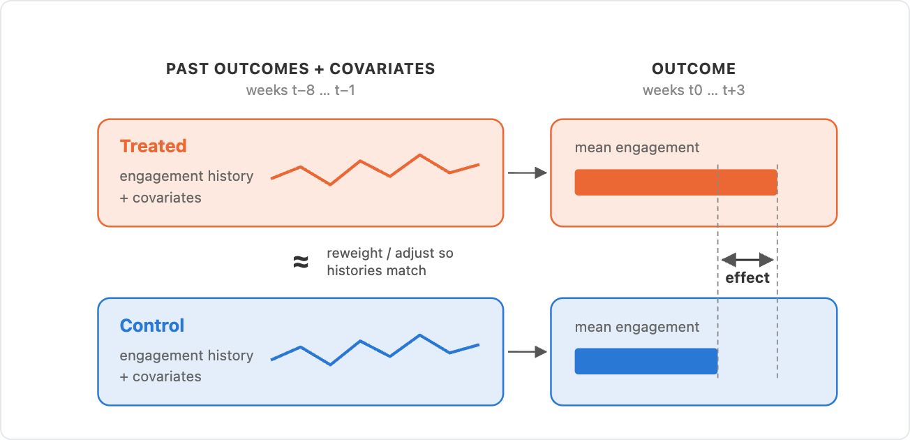
Lagged-outcome regression compares handled and management customers who had the identical engagement historical past and traits earlier than remedy. After re-weighting or adjusting so these histories match, the distinction in post-period engagement is the impact.

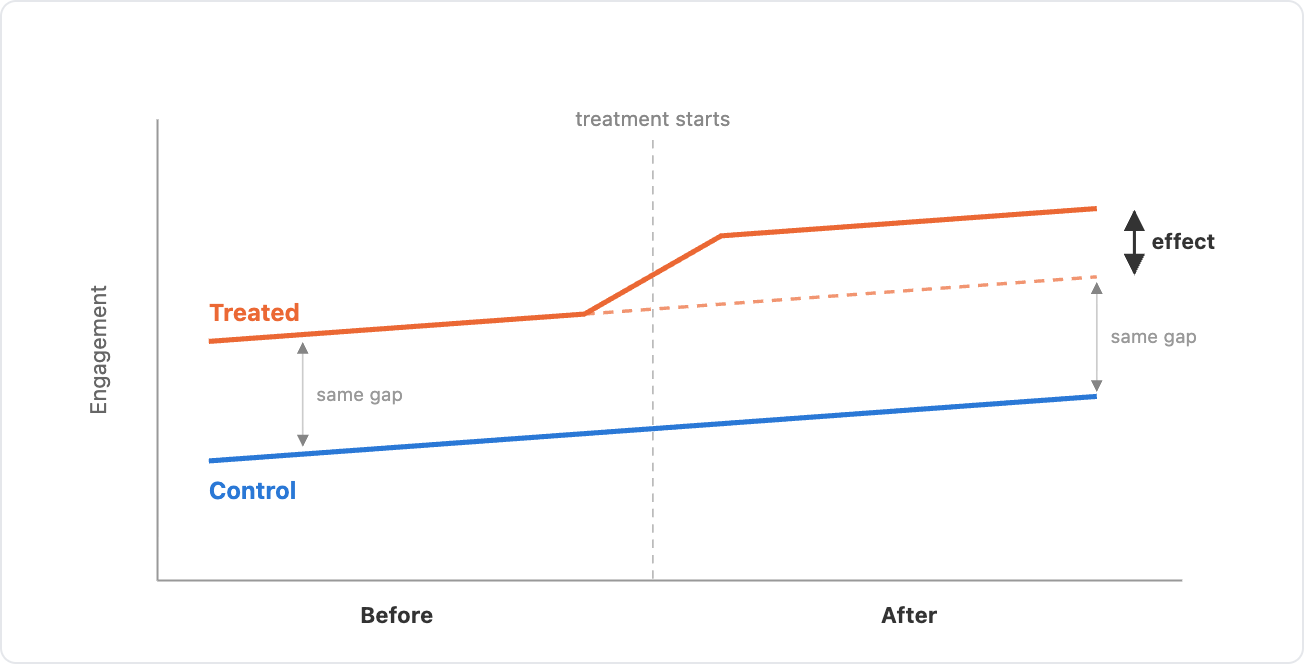
Distinction-in-differences lets the 2 teams begin at totally different ranges. It assumes the hole between them would have stayed the identical with out remedy, so any change within the hole after remedy is the impact. In observe DiD is often conditional: parallel traits solely want to carry amongst customers with the identical traits, measured earlier than the pre-period.

Lagged-outcome regression could be estimated by regression adjustment, inverse propensity weighting or double machine studying. Distinction-in-differences has the identical menu, from two-way fastened results to doubly strong DiD.

Doubly strong means the estimate survives a flawed consequence mannequin or a flawed propensity mannequin. It does nothing if the figuring out assumption fails.

A helpful option to see the distinction is to put in writing the post-period consequence as a perform of the pre-period consequence:

Right here D is the remedy, τ the impact and X the noticed covariates. τ is the handled–management hole after adjusting for Y_pre and X.

• Distinction-in-differences units β = 1. Subtract Y_pre from either side and τ turns into the handled–management distinction in every consumer’s change. This treats each pre-period hole as everlasting: no matter separated the teams earlier than remedy carries into the post-period in full.

• Lagged-outcome regression estimates β. Pre-period engagement mixes a long-lasting stage with short-term shocks that fade, reminiscent of a busy week or a vacation, so the estimate lands beneath 1. This treats a part of each pre-period hole as short-term: a bunch that began low is predicted to recuperate partly by itself.

Every design is biased when the hole between the teams will not be the sort it assumes. That occurs in two frequent conditions.

2. Two failure modes

Failure mode 1: a time-invariant confounder

Take a free trial of a premium tier. Greater-income customers usually tend to begin it, they usually additionally have a tendency to interact extra each week. Earnings not often adjustments over a couple of months and is often not in your knowledge. That makes it an unobserved, time-invariant confounder.

DiD handles this: a relentless distinction between customers cancels whenever you subtract the pre-period. Lagged-outcome regression can solely regulate for revenue so far as previous engagement reveals it, so a part of the distinction leads to the estimate.

Failure mode 2: choice on a short lived dip

Customers usually choose in when one thing has simply modified. Take a win-back marketing campaign: customers whose exercise has slipped are provided a free trial of a premium tier, and those who settle for are disproportionately in a short lived stoop. A lot of them would have bounced again anyway. Ashenfelter (1978) discovered the identical sample in job coaching: trainees’ earnings fall simply earlier than they enrol and recuperate afterwards, whether or not the coaching labored or not.

DiD subtracts every consumer’s pre-period, and its covariates are measured earlier than it, so nothing within the design accounts for the dip. The pre-period is depressed, and the restoration is counted as a part of the impact. A dip that hits handled and management customers alike, reminiscent of a vacation week, will not be an issue, as a result of the management change absorbs it. Lagged-outcome regression situations on the dip itself: it compares dipped handled customers with controls who dipped the identical manner.

To measure these biases we want knowledge the place the true impact is thought, so the subsequent part simulates it.

3. A simulation with a identified reply

The simulation builds a weekly panel of 10,000 customers. Every consumer’s weekly engagement (suppose minutes per week, round 30 for a typical consumer) is the sum of 4 elements:

• a stage set by noticed covariates and an unobserved time-invariant confounder

• a pattern that is dependent upon the noticed covariates

• seasonality shared by everybody

• a short lived shock that fades by 20% every week

Each consumer will get a candidate week. Handled customers choose in that week, and controls are customers who have been eligible that week and didn’t. The function provides 2 minutes every week for each handled consumer, so the true impact is 2.0. Engagement with and with out the function is simulated for each consumer, which is what lets us plot the true counterfactual beneath.

What adjustments between situations is why customers choose in. In each state of affairs, customers with decrease engagement usually tend to choose in.

The 4 choice situations

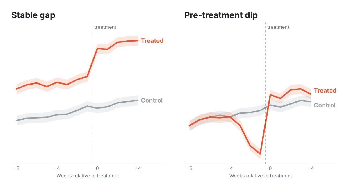
The uncooked knowledge exhibits every mechanism: in a, the teams differ solely by noticed covariates; in b, handled customers sit decrease each week however transfer in parallel; in c, handled customers dip within the three weeks earlier than opting in; d has each.

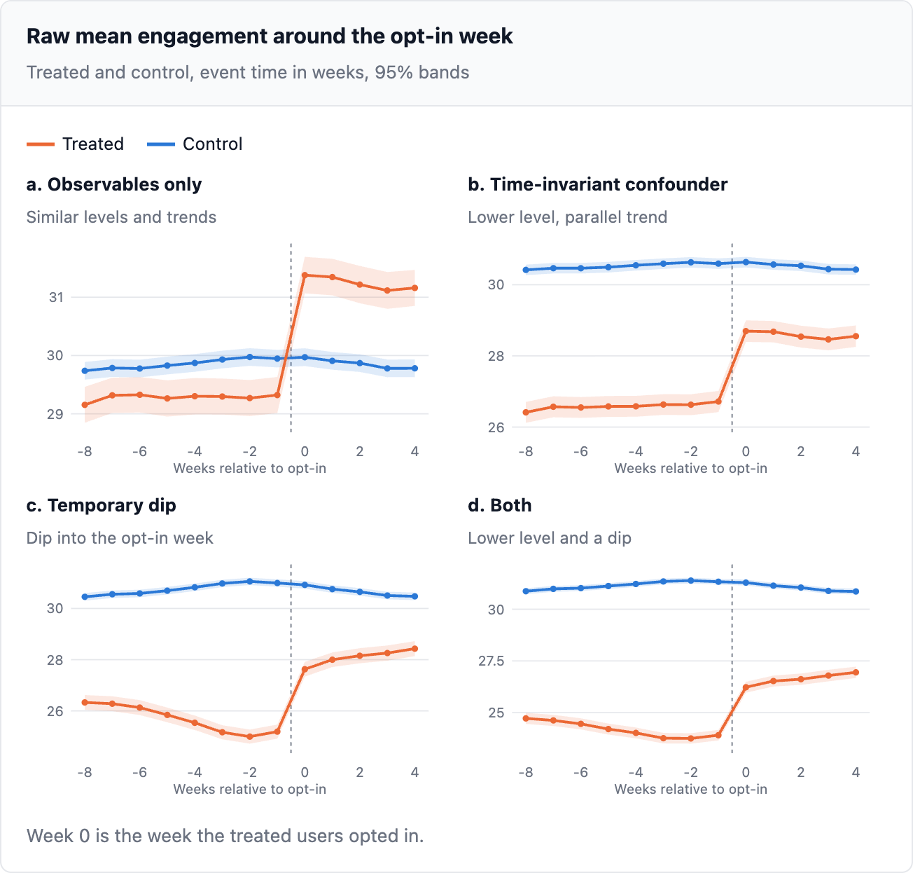
On every dataset each designs are estimated the identical manner, with double machine studying in DoubleML. Lagged-outcome regression makes use of DoubleMLIRM with the ATTE rating on imply engagement in weeks 0 to three. DiD makes use of DoubleMLDIDBinary on the imply over the baseline window (weeks -4 to -1) and the post-period imply (weeks 0 to three). Each use LightGBM for the result and propensity fashions, five-fold cross-fitting and propensities clipped at 0.01.

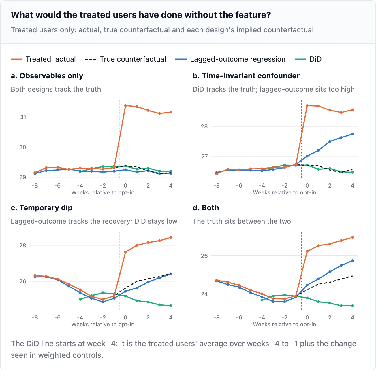
The following chart exhibits the handled customers solely. Orange is what they did, black dashed is what they might have carried out with out the function, and every colored line is what a design assumes they might have carried out. A design’s estimate is the hole between orange and its personal line after week 0.

• a. Each traces sit on the true counterfactual. Each estimates are proper.

• b. DiD tracks the reality. The lagged-outcome line rises after week 0 as a result of its matched controls drift again up (failure mode 1), so it understates the impact.

• c. The true counterfactual climbs again because the dip wears off. Lagged-outcome regression follows it. DiD stays on the dipped baseline (failure mode 2), so it overstates the impact.

• d. The lagged-outcome line sits above the reality and the DiD line beneath it. One estimate is simply too small and the opposite too giant, so the reality sits between them.

One dataset exhibits one draw. To see the everyday estimate and its unfold, every state of affairs was simulated 200 instances and each designs have been estimated on each replication.

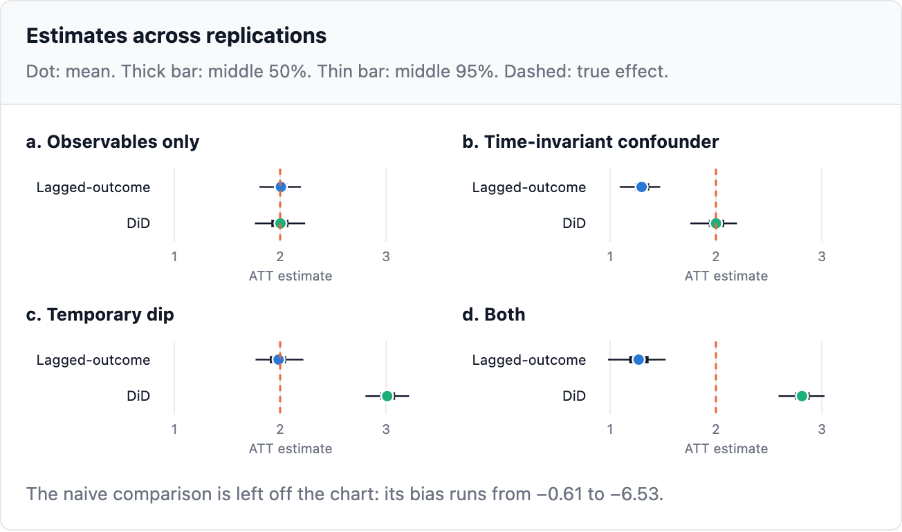
Every design is unbiased the place its assumption holds and badly biased the place it doesn’t. The biased designs additionally had slim intervals. In state of affairs b, DiD’s 95% intervals contained the true impact in 94% of replications and lagged-outcome regression’s in 0%. Nothing within the output warns you.

Lagged-outcome regression handles the dip as a result of it situations on the lagged outcomes. So cannot we repair DiD by including lagged outcomes to it too?

4. Can previous engagement repair DiD?

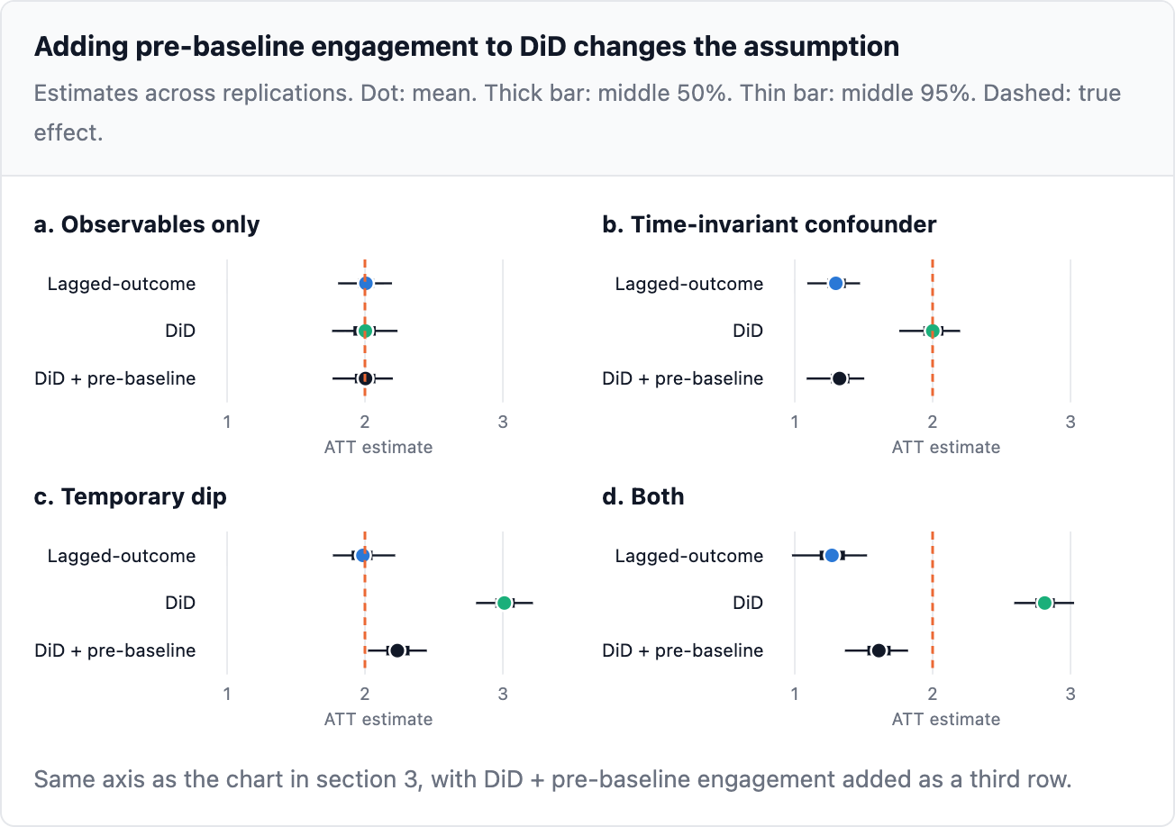
A standard intuition is to present DiD extra of every consumer’s historical past by including their engagement in weeks -8 to -5, earlier than the baseline window, as covariates. Daw and Hatfield (2018) confirmed this will backfire: when the teams differ in stage, matching on previous outcomes pairs handled customers with controls whose engagement was briefly uncommon, and people controls drift again in the direction of their very own imply. The examine measures the fee with a 3rd design, DiD + pre-baseline engagement.

• Situation b: parallel traits holds, and including pre-baseline engagement makes DiD about as biased as lagged-outcome regression (−0.68, in opposition to −0.70 for lagged-outcome regression and +0.00 for plain DiD).

• Situation c: it helps, as a result of it carries a part of the dip, however it doesn’t take away the bias (+0.23 in opposition to +1.01).

• Situation d: it lands at −0.39, in opposition to −0.73 for lagged-outcome regression and +0.81 for plain DiD.

So it solely helps the place parallel traits already fails, and there the pre-trend verify sends you to lagged-outcome regression, which handles the dip totally. Its end in d is closest to the reality solely as a result of two biases occur to partially cancel. The place the pre-trend is flat and DiD is the fitting design, it could actually solely harm.

That provides one covariate rule per design:

• Lagged-outcome regression: situation on the result historical past. Right here that’s engagement in every of the eight weeks earlier than opt-in, its slope and the newest change, plus the non-outcome covariates.

• DiD: use non-outcome covariates measured earlier than the baseline window, and no pre-baseline engagement or different consequence historical past.

5. The diagnostic: verify the pre-trend

To decide on between the designs, have a look at the pre-period. Nothing has been handled but, so any distinction between handled and management there comes from choice (assuming customers don’t change behaviour in anticipation of opting in).

The pre-trend verify

Consider the verify as working the DiD one window early. Weeks -8 to -5 play the baseline and weeks -4 to -1 play the post-period. Nobody is handled but, so if parallel traits holds the “impact” there may be zero. A confounder that solely shifts a consumer’s stage cancels out, precisely because it does in DiD, so b stays flat. A dip doesn’t: throughout replications, the hole in c averages −1.33 over weeks -4 to -1. That’s the identical dip DiD later counts as a part of the impact when it recovers (a bias of +1.01).

The verify mirrors the DiD design:

1. Take every consumer’s common engagement in weeks -8 to -5 as their reference stage, and subtract it from each later week. This removes stage variations, as DiD does.

2. Weight the controls on the non-outcome covariates solely, because the DiD design does.

3. Plot the handled minus weighted-control hole week by week. If parallel traits holds, it stays flat at zero by weeks -4 to -1.

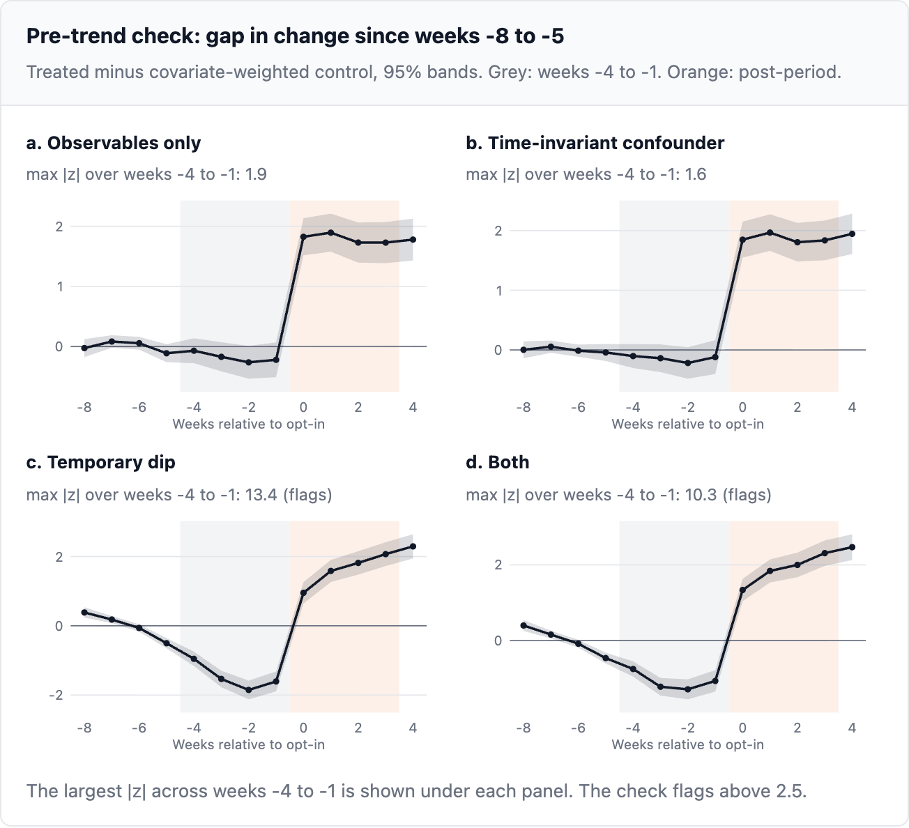
Flat in a and b, a transparent dip in c and d. Parallel traits fails precisely the place DiD was biased. Throughout the replications the verify flagged each run of c and d, and three% of a and three% of b. The two.5 threshold retains the false alarm charge close to 5% throughout the 4 weeks.

A flat pre-trend helps parallel traits however doesn’t show it: the verify can not see something that begins at opt-in, reminiscent of a shock that week or customers performing in anticipation, or a dip older than the window. And with fewer customers or noisier engagement an actual violation can move, which makes estimates reported solely after a passing verify much less dependable than they appear (Roth 2022).

6. The choice rule

A failed verify guidelines out this DiD, not each DiD. If the dip is brief, a pre-period that ends earlier than it could actually nonetheless work, and sensitivity strategies reminiscent of Rambachan and Roth (2023) present how far the estimate strikes if parallel traits is violated by a bounded quantity.

In observe, report each. When the verify dips, DiD continues to be value reporting, as a result of the 2 estimates certain the reality (see the FAQ beneath). In the event that they result in the identical resolution, the selection of design does not matter. In the event that they straddle zero or your resolution threshold, the info cannot settle it.

Continuously requested questions

Is there a pre-trend verify for lagged-outcome regression?

The usual one is a placebo, additionally referred to as a pseudo-outcome check (Imbens and Rubin 2015): match the mannequin on historical past as much as week -5 and estimate the “impact” on weeks -4 to -1, the place it needs to be zero. Drawn the identical manner because the DiD verify, it seems to be like this:

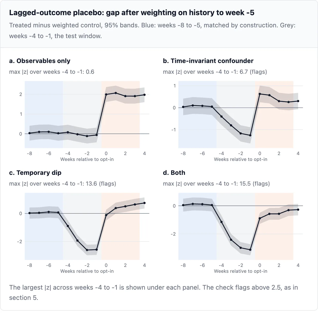
Learn it just like the DiD verify: flat by weeks -4 to -1 helps the design. It caught the confounder in b, with a placebo estimate of −0.80 throughout replications in opposition to an actual bias of −0.70. But it surely additionally bends in c, the place lagged-outcome regression is correct, as a result of these customers opted in primarily based on weeks -3 to -1, which a mannequin stopped at week -5 can not see. So it can not select between the designs. Its use is narrower: when the pre-trend verify is flat, it tells you whether or not lagged-outcome regression would have agreed with DiD.

Becoming on the complete historical past to week -1 doesn’t assist. Each pre-period week then matches by building, so the chart exhibits the impact over time however exams nothing.

Conclusion

The identical estimator was utilized in each designs. The fitting one was whichever assumption matched how customers opted in.

• Separate the estimator from the design. DML is the way you estimate. Whether or not the estimate is causal is dependent upon unconfoundedness or parallel traits holding.

• Let the pre-trend select. Flat: DiD. Dip: lagged-outcome regression, with DiD as the opposite certain.

The simulation exhibits that every design fails in a predictable state of affairs, {that a} biased design nonetheless produces tight intervals, and that the pre-trend verify picks out the dip. It doesn’t present how usually every state of affairs happens in actual merchandise. It makes use of one data-generating course of, choice in the direction of much less engaged customers, one estimator library, and an consequence that isn’t absorbing. By yourself knowledge, begin with how customers got here to choose in, then have a look at the pre-trend.

The simulator, estimators and diagnostics are within the companion repo, together with a pocket book that reproduces each determine right here. The diagnostics take a protracted panel with your individual column names, so the checks in part 5 run on actual knowledge unchanged.

References

• Angrist, J. and Pischke, J.-S. (2009). Largely Innocent Econometrics, part 5.4. Princeton College Press.

• Ashenfelter, O. (1978). Estimating the impact of coaching applications on earnings. Assessment of Economics and Statistics, 60(1), 47–57.

• Chernozhukov, V. et al. (2018). Double/debiased machine studying for remedy and structural parameters. The Econometrics Journal, 21(1), C1–C68.

• Chernozhukov, V. et al. (2022). Lengthy story brief: omitted variable bias in causal machine studying. NBER Working Paper 30302.

• Daw, J. and Hatfield, L. (2018). Matching and regression to the imply in difference-in-differences evaluation. Well being Companies Analysis, 53(6), 4138–4156.

• Ding, P. and Li, F. (2019). A bracketing relationship between difference-in-differences and lagged-dependent-variable adjustment. Political Evaluation, 27(4), 605–615.

• Imbens, G. and Rubin, D. (2015). Causal Inference for Statistics, Social, and Biomedical Sciences, chapter “Assessing unconfoundedness”. Cambridge College Press.

• Rambachan, A. and Roth, J. (2023). A extra credible strategy to parallel traits. Assessment of Financial Research, 90(5), 2555–2591.

• Roth, J. (2022). Pretest with warning: event-study estimates after testing for parallel traits. American Financial Assessment: Insights, 4(3), 305–322.

• Sant’Anna, P. and Zhao, J. (2020). Doubly strong difference-in-differences estimators. Journal of Econometrics, 219(1), 101–122.

Simulated knowledge all through. Each chart and quantity on this web page is generated by instruments/article_data.py within the companion repo, besides the robustness values within the FAQ, which come from the pocket book.

···

Ryan O’Sullivan is a lead knowledge scientist with over 16 years’ expertise in causal inference and advertising and marketing combine modelling. Comply with him on LinkedIn for extra on advertising and marketing measurement.

···

*All photographs have been created by the creator utilizing Claude and HTML.