The theoretical case for autoencoders
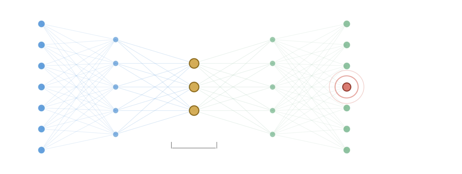
Autoencoders — neural networks educated to reconstruct their very own enter by means of a compressed bottleneck — are an ordinary advice for anomaly detection. The theoretical argument is clear: prepare the community solely on regular information, and it learns to reconstruct regular patterns properly. Feed it an anomaly, and reconstruction error spikes, as a result of the community by no means realized to compress that form of sample. Not like PCA, which may solely seize linear relationships between options, an autoencoder can in precept study nonlinear ones — so it ought to catch anomalies that violate a nonlinear construction within the information, which a linear technique structurally can’t.
That is a particular, testable declare, not a imprecise one: autoencoders ought to have an actual, measurable edge over PCA particularly on anomalies that violate nonlinear relationships. So I constructed two experiments — one simple case, and one intentionally designed to be the autoencoder’s finest shot — and measured whether or not the theoretical benefit really exhibits up.
Setup, each experiments: artificial information (clearly labeled as such — this isn’t an actual sensor or fraud dataset), educated on regular samples solely (the real looking anomaly-detection setup — you not often have labeled anomalies to coach on), evaluated on a held-out mixture of regular and anomalous samples. Three strategies in contrast: an autoencoder (MLPRegressor educated to reconstruct its personal enter, with a third-dimensional bottleneck), PCA reconstruction error (additionally lowered to three parts — similar bottleneck measurement, for a good comparability), and Isolation Forest as a non-reconstruction-based reference level.
Experiment 1: the straightforward case
Regular information drawn from a combination of Gaussian clusters (representing, say, a couple of regular working regimes of a machine). Anomalies drawn from a distribution with a shifted imply and better variance — an easy, linearly-separable form of outlier.
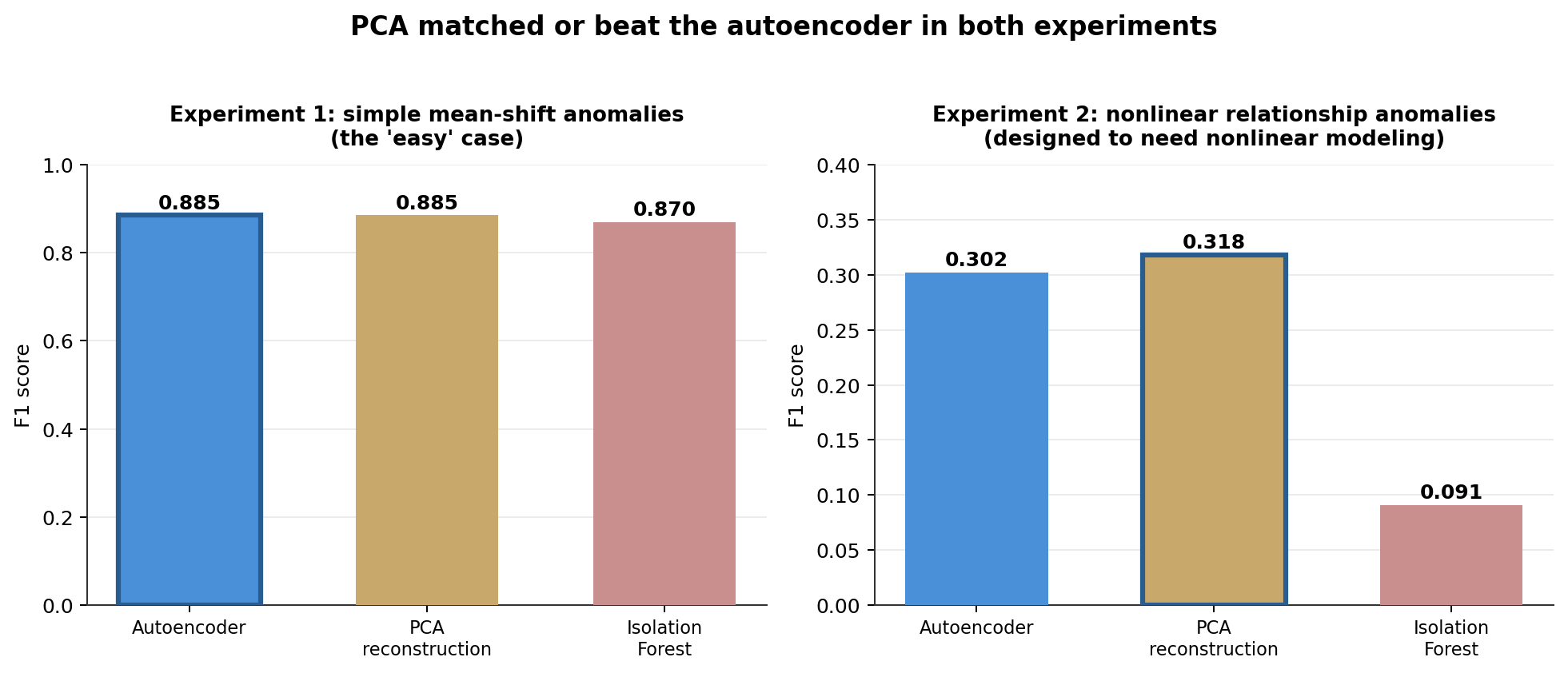
Autoencoder and PCA tied precisely — 0.885 F1, each catching each single anomaly (recall = 1.0), differing solely barely on precision. Isolation Forest got here in simply behind at 0.870. This outcome alone is not stunning as soon as you concentrate on why: a imply shift is a linear phenomenon, so a linear technique has no structural drawback detecting it. The autoencoder’s further representational capability was merely pointless right here.
This is why it was really easy — the precise reconstruction error distribution the autoencoder produced on the take a look at set:
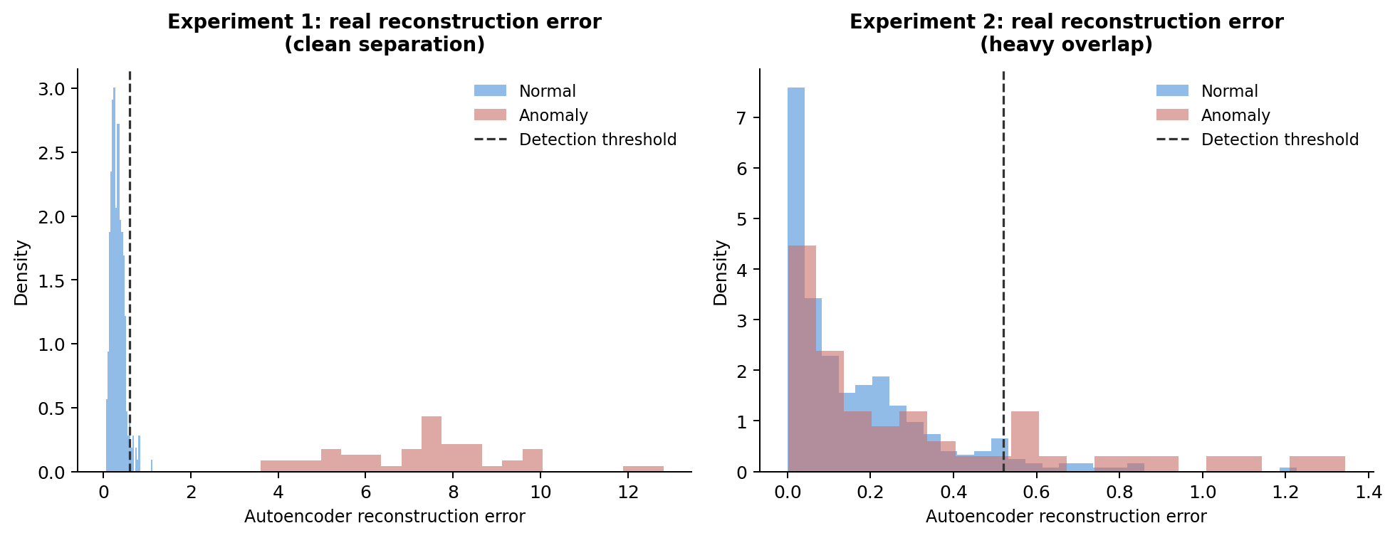
In Experiment 1 (left panel), regular and anomalous reconstruction errors barely overlap in any respect — regular samples cluster tightly beneath 1.0, anomalies sit virtually completely above 4.0. Any cheap threshold in that hole catches all the pieces. That is what “simple” seems like in reconstruction-error phrases, and it explains why a linear technique does simply in addition to a nonlinear one: the separation is giant sufficient that neither technique’s precision issues a lot.
Experiment 2: rigging the take a look at within the autoencoder’s favor
That is the half that really exams the theoretical declare. I constructed anomalies particularly designed to be invisible to a linear technique: regular information the place two options observe a nonlinear relationship (y = sin(3x) + noise), and anomalies that hold the similar particular person vary for every function however violate the connection between them — x and y every look completely regular in isolation; solely their joint, nonlinear relationship is fallacious. That is near a best-case situation for an autoencoder’s theoretical benefit: a sample a linear projection genuinely can’t signify, by building.
The autoencoder nonetheless did not win. PCA scored 0.318 F1, the autoencoder scored 0.302 — PCA very barely forward, each far weaker than Experiment 1 (which is smart — it is a genuinely tougher detection drawback for any technique) however with no autoencoder benefit wherever in sight. Isolation Forest fell aside completely on this job, at 0.091.
The correct panel of the histogram above exhibits why this one was laborious for everybody: regular and anomalous reconstruction errors overlap closely, with no clear hole to threshold on. Some anomalies produced decrease reconstruction error than loads of regular samples — that means no fastened threshold, on both technique’s error sign, may have separated them cleanly. That is a materially completely different failure mode than “the fallacious technique was used” — it is “the detection sign itself did not separate the lessons properly,” which is a knowledge and modeling-choice drawback, not merely a which-algorithm drawback.
Why the theoretical benefit did not present up
This is not proof that autoencoders cannot outperform PCA — it is proof that an untuned, default-architecture autoencoder does not routinely notice its theoretical benefit, and that hole between idea and default observe is the precise discovering price taking severely.
A number of concrete causes this probably occurred:
-
700 coaching samples isn’t a lot information for a neural community to study a nonlinear manifold from scratch. PCA’s linear answer has a closed-form optimum computable from a handful of samples; the autoencoder has to discover a good nonlinear answer by gradient descent, which wants meaningfully extra information to do reliably.
-
A single default structure (8-3-8,
max_iter=2000) is a beginning guess, not a tuned mannequin. Capturing a particular nonlinear relationship properly typically requires intentionally shaping the structure across the form of nonlinearity anticipated — completely different depth, width, activation operate, or coaching period — none of which I searched over right here. -
Reconstruction-error anomaly detection has a structural limitation that hits each strategies: when the anomaly sign is concentrated in a subset of options and diluted by averaging throughout all of them, each linear and nonlinear reconstruction error can miss it. I noticed this straight in an earlier model of this experiment with extra noise dimensions, the place each strategies collapsed to near-random efficiency — a separate, helpful lesson about reconstruction-based detection in high-dimensional settings.
What would really be wanted to unlock the autoencoder’s benefit right here? A number of concrete, testable subsequent steps, in tough order of how low-cost they’re to strive: improve coaching information quantity considerably (the nonlinear relationship wants sufficient examples to be learnable, not simply theoretically learnable); widen or deepen the structure particularly across the 2 options carrying the sign moderately than a generic 8-3-8 form; examine the realized bottleneck illustration straight (plot the three bottleneck activations, coloured by true label) to see whether or not the anomalies are even separable in that latent area, which might inform you whether or not the issue is illustration or thresholding; and contemplate a feature-weighted reconstruction error, so the 2 informative options aren’t averaged down by uninformative ones. None of those are unique — they’re the precise engineering work “simply add an autoencoder” skips over.
The precise choice framework
Earlier than reaching for an autoencoder over an easier reconstruction-based technique like PCA, three questions are price answering first:
-
Does your information have genuinely nonlinear relationships between options, or does it simply really feel prefer it ought to? “Complicated-sounding information” and “information with nonlinear construction a linear technique cannot seize” aren’t the identical factor — confirm the second particularly earlier than assuming it justifies the additional mannequin complexity.
-
Do you have got sufficient normal-only coaching information for a neural community to really study that construction? PCA’s linear answer is almost data-efficient by building; a neural community’s nonlinear answer typically is not. A number of hundred samples is likely to be loads for PCA and never almost sufficient for a community to search out actual sign as a substitute of noise.
-
Have you ever really regarded on the reconstruction error distribution, for both technique, earlier than trusting both one’s threshold? A histogram like those above takes one line of code and tells you instantly whether or not you are coping with a clear separation drawback (the place the selection of technique barely issues) or a real overlap drawback (the place neither technique’s threshold will prevent with out extra elementary modifications).
The place this comparability falls quick
-
Artificial information, intentionally constructed — each experiments use information I generated particularly to check a speculation, not actual sensor or fraud information. The qualitative lesson (default architectures do not routinely ship their theoretical benefit) is extra more likely to generalize than the precise numbers.
-
One structure, one coaching run. I did not search over autoencoder depth, width, or coaching period — which is exactly the purpose (this text exams the “simply use an autoencoder” default, not the ceiling of what a well-tuned one can do), however it means these outcomes describe the default, not the most effective case.
-
A single random seed for the anomaly technology. Totally different artificial anomaly constructions may shift these particular numbers; the path — no autoencoder benefit materializing by default — is the extra strong a part of the discovering.
Conclusion
“Autoencoders can mannequin nonlinear relationships that PCA cannot” is true as a press release about representational capability. It’s not the identical declare as “an autoencoder will outperform PCA in your anomaly detection job by default” — and conflating the 2 is the place the sensible disappointment comes from. Realizing a neural community’s theoretical benefit over an easier linear technique takes actual tuning effort, actual information quantity, and actual structure selections; none of that comes free of charge simply from selecting the extra highly effective mannequin class. Earlier than reaching for the autoencoder, it is price asking the identical query that applies to each “fancier technique” choice: does the development present up once you really measure it, or solely once you assume it ought to?