


Bayesian statistics you’ve seemingly encountered MCMC. Whereas the remainder of the world is fixated on the newest LLM hype, Markov Chain Monte Carlo stays the quiet workhorse of high-end quantitative finance and threat administration. It’s the device of selection when “guessing” isn’t sufficient and it’s good to rigorously map out uncertainty.
Regardless of the intimidating acronym, Markov Chain Monte Carlo is a mix of two easy ideas:
- A Markov Chain is a stochastic course of the place the following state of the system relies upon totally on its present state and never on the sequences of occasions that preceded it. This property is often known asmemorylessness.
- A Monte Carlo methodology merely refers to any algorithm that depends on repeated random sampling to acquire numerical outcomes.
On this collection, we are going to current the core algorithms utilized in MCMC frameworks. We primarily concentrate on these used for Bayesian strategies.
We start with Metropolis-Hastings: the foundational algorithm that enabled the sphere’s earliest breakthroughs. However earlier than diving into the mechanics, let’s focus on the issue MCMC strategies assist remedy.
The Downside
Suppose we wish to have the ability to pattern variables from a likelihood distribution which we all know the density components for. On this instance we use the usual regular distribution. Let’s name a operate that may pattern from it rnorm.
For rnorm to be thought-about useful, it should generate values (x) over the long term that match the possibilities of our goal distribution. In different phrases, if we had been to let rnorm run (100,000) instances and if we had been to gather these values and plot them by the frequency they appeared (a histogram), the form would resemble the usual regular distribution.
How can we obtain this?
We begin with the components for the unnormalised density of the traditional distribution:
[p(x) = e^{-frac{x^2}{2}}]
This operate returns a density for a given (x) as a substitute of a likelihood. To get a likelihood, we have to normalise our density operate by a relentless, in order that the whole space beneath the curve integrates (sums) to (1).
To seek out this fixed we have to combine the density operate throughout all potential values of (x).
[C = int^infty_{-infty}e^{-frac{x^2}{2}},dx]
There is no such thing as a closed-form answer to the indefinite integral of (e^{-x^2}). Nonetheless, mathematicians solved the particular integral (from (-infty) to (infty)) by transferring to polar coordinates (as a result of apparently, turning a (1D) drawback to a (2D) one makes it simpler to unravel) , and realising the whole space is (sqrt{2pi}).
Subsequently, to make the world beneath the curve sum to (1), the fixed should be the inverse:
[C = frac{1}{sqrt{2pi}}]
That is the place the well-known normalisation fixed (C) for the traditional distribution comes from.
OK nice, we’ve got the mathematician-given fixed that makes our distribution a legitimate likelihood distribution. However we nonetheless want to have the ability to pattern from it.
Since our scale is steady and infinite the likelihood of getting precisely a particular quantity (e.g. (x = 1.2345…) to infinite precision) is definitely zero. It is because a single level has no width, and subsequently accommodates no ‘space’ beneath the curve.
As an alternative, we should communicate when it comes to ranges i.e. what’s the likelihood of getting a worth (x) that falls between (a) and (b) ((a < x < b)), the place (a) and (b) are fastened values?
In different phrases, we have to discover the world beneath the curve between (a) and (b). And as you’ve accurately guessed, to calculate this space we sometimes have to combine our normalised density components – the ensuing built-in operate is named the Cumulative Distribution Perform ((CDF)).
Since we can’t remedy the integral, we can’t derive the (CDF) and so we’re caught once more. The intelligent mathematicians solved this too and have been in a position to make use of trigonometry (particularly the Field-Muller rework) to transform uniform random variables to regular random variables.
However right here is the catch: In the actual world of Bayesian statistics and machine studying, we take care of advanced multi-dimensional distributions the place:
- We can’t remedy the integral analytically.
- Subsequently we can’t discover the normalisation fixed (C)
- Lastly, with out the integral, we can’t calculate the CDF, so normal sampling fails.
We’re caught with an unnormalised components and no solution to calculate the whole space. That is the place MCMC is available in. MCMC strategies enable us to pattern from these distributions with out ever needing to unravel that unattainable integral.
Introduction
A Markov course of is uniquely outlined by its transition possibilities (P(xrightarrow x’)).
For instance in a system with (4) states:
[P(xrightarrow x’) = begin{bmatrix} 0.5 & 0.3 & 0.05 & 0.15 0.2 & 0.4 & 0.1 & 0.3 0.4 & 0.4 & 0 & 0.2 0.1 & 0.8 & 0.05 & 0.05 end{bmatrix}]
The likelihood of going from any state (x) to (x’) is given by entry (i rightarrow j) within the matrix.
Have a look at the third row, as an example: ([0.4,0.4,0,0.2]).
It tells us that if the system is at present in State (3), it has a (40%) likelihood of transferring to State (1), a (40%) likelihood of transferring to State (2), a (0%) likelihood of staying in State (3), and a (20%) likelihood of transferring to State (4).
The matrix has mapped each potential path with its corresponding possibilities. Discover that every row (i) sums to (1) in order that our transition matrix represents legitimate possibilities.
A Markov course of additionally requires an preliminary state distribution (pi_0) (can we begin in state (1) with (100%) likelihood or any of the (4) states with (25%) likelihood every?).
For instance, this might appear like:
[pi_0 = begin{bmatrix} 0.4 & 0.15 & 0.25 & 0.2 end{bmatrix}]
This merely means the likelihood of ranging from state (1) is (0.4), state (2) is (0.15) and so forth.
To seek out the likelihood distribution of the place the system will likely be after step one (t_0 + 1), we multiply the preliminary distribution with the transition possibilities:
[ pi_1 = pi_0P]
The matrix multiplication successfully offers us the likelihood of all of the routes we are able to take to get to a state (j) by summing up all the person possibilities of reaching (j) from completely different beginning states (i).
Why this works
By utilizing matrix multiplication we’re exploring each potential path to a vacation spot and summing their chance.
Discover that the operation additionally superbly preserves the requirement that the sum of the possibilities of being in a state will all the time equal (1).
Stationary Distribution
A correctly constructed Markov course of reaches a state of equilibrium because the variety of steps (t) approaches infinity:
[pi^* P = pi^*]
Such a state is named world steadiness.
(pi^*) is named the stationary distribution and represents a time at which the likelihood distribution after a transition ((pi^*P)) is equivalent to the likelihood distribution earlier than the transition ((pi^*)).
The existence of such a state occurs to be the inspiration of each MCMC methodology.
When sampling a goal distribution utilizing a stochastic course of, we aren’t asking “The place to subsequent?” however relatively “The place can we find yourself ultimately?”. To reply that, we have to introduce long run predictability into the system.
This ensures that there exists a theoretical state (t) at which the possibilities “settle” down as a substitute of transferring in random for all eternity. The purpose at which they “settle” down is the purpose at which we hope we are able to begin sampling from our goal distribution.
Thus, to have the ability to successfully estimate a likelihood distribution utilizing a Markov course of we have to be sure that:
- there exists a stationary distribution.
- this stationary distribution is distinctive, in any other case we may have a number of states of equilibrium in an area far-off from our goal distribution.
The mathematical constraints imposed by the algorithm make a Markov course of fulfill these situations, which is central to all MCMC strategies. How that is achieved might fluctuate.
Uniqueness
Typically, to ensure the distinctiveness of the stationary distribution, we have to fulfill three situations. Develop the part under to see them:
The Holy Trinity
- Irreducible: A system is irreducible if at any state (x) there’s a non-zero likelihood of any level (x’) within the pattern house being visited. Merely put, you will get from any state A to any state B, ultimately.
- Aperiodic: The system should not return to a specific state in fastened intervals. A adequate situation for aperiodicity is that there exists not less than one state the place the likelihood of staying is non-zero.
- Optimistic Recurrent: A state (x) is optimistic recurrent if ranging from that state the system is assured to return to it and the typical variety of steps it takes to return to is finite. That is assured by us modelling a goal that has a finite integral and is a correct likelihood distribution (the world beneath the curve should sum to (1)).
Any system that meets these situations is named an ergodic system. The tables on the finish of the article present how the MH algorithm offers with making certain ergodicity and subsequently uniqueness.
Metropolis-Hastings
The method the MH algorithm takes is to start with the definition of detailed steadiness – a adequate however not not mandatory situation for world steadiness. Fairly merely, if our algorithm satisfies detailed steadiness, we are going to assure that our simulation has a stationary distribution.
Derivation
The definition of detailed steadiness is:
[pi(x) P(x’|x) = pi(x’) P(x|x’) ,]
which means the likelihood circulation of going from (x) to (x’) is identical because the likelihood circulation going from (x’) to (x).
The thought is to seek out the stationary distribution by iteratively constructing the transition matrix, (P(x’,x)) by setting (pi) to be the goal distribution (P(x)) we wish to pattern from.
To implement this, we decompose the transition likelihood (P(x’|x)) into two separate steps:
- Proposal ((g)): The likelihood of proposing a transfer to (x’) given we’re at (x).
- Acceptance ((A)): The acceptance operate offers us the likelihood of accepting the proposal.
Thus,
[P(x’|x) = g(x’|x) a(x’,x)]
The Hastings Correction
Substituting these values again into the equation above offers us:
[frac{pi(x)}{pi(x’)} = fracx’) a(x,x’)x) a(x’,x)]
and at last rearranging we get an expression for our acceptance as a ratio:
[frac{a(x’,x)}{a(x,x’)} = fracx’)pi(x’)x)pi(x)]
This ratio represents how more likely we’re to just accept a transfer to (x’) in comparison with a transfer again to (x).
The (fracx’)pi(x’)x)pi(x)) time period is named the Hastings correction.
Essential Word
As a result of we regularly select a symmetric distribution for the proposal, the likelihood of leaping from (x rightarrow x’) is identical as leaping from (x’ rightarrow x). Subsequently, the proposal phrases cancel one another out leaving solely the ratio of the goal densities.
This particular case the place the proposal is symmetric and the (g) phrases vanish is traditionally often called the Metropolis Algorithm (1953). The extra normal model that enables for uneven proposals (requiring the (g) ratio – often called the Hastings correction) is the Metropolis-Hastings Algorithm (1970).
The Breakthrough
Recall the unique drawback: we can’t calculate (pi(x)) as a result of we don’t know the normalisation fixed (C) (the integral).
Nonetheless, look carefully on the ratio (frac{pi(x’)}{pi(x)}). If we develop (pi(x)) into its unnormalised density (f(x)) and the fixed (C):
[frac{pi(x’)}{pi(x)} = frac{{f(x’)} / C}{f(x) / C} = frac{f(x’)}{f(x)}]
The fixed (C) cancels out!
That is the breakthrough. We will now pattern from a posh distribution utilizing solely the unnormalised density (which we all know) and the proposal distribution (which we select).
All that’s left to do is to seek out an acceptance operate (A) that may fulfill detailed steadiness:
[frac{a(x’,x)}{a(x,x’)} = R ,]
the place (R) represents (fracx’)pi(x’)x)pi(x)).
The Metropolis Acceptance
The acceptance operate the algorithm makes use of is:
[a(x’,x) = min(1,R)]
This ensures that the acceptance likelihood is all the time between (0) and (1).
To see why this selection satisfies detailed steadiness, we should confirm that the equation holds for the reverse transfer as effectively. We have to confirm that:
[frac{a(x’,x)}{a(x,x’)} = R,]
in two circumstances:
Case I: The transfer is advantageous ((R ge 1))
Since (R ge 1), the inverse (frac{1}{R} le 1):
- our ahead acceptance is (a(x’,x) = min(1,R) = 1)
- our reverse acceptance is (a(x,x’) = min(1,frac{1}{R}) = frac{1}{R})
[frac{1}{a(x,x’)} = R]
[frac{1}{frac{1}{R}} = R]
Case II: The transfer will not be advantageous ((R < 1))
Since (R < 1), the inverse (frac{1}{R} > 1):
- our ahead acceptance is (a(x’,x) = min(1,R) = R)
- our reverse acceptance is (a(x,x’) = min(1,frac{1}{R}) = 1)
Thus:
[frac{R}{a(x,x’)} = R]
[frac{R}{1} = R,]
and the equality is glad in each circumstances.
Implementation
Lets implement the MH algorithm in python on two instance goal distributions.
I. Estimating a Gaussian Distribution
After we plot the samples on a chart in opposition to a real regular distribution that is what we get:

Now you may be pondering why we bothered working a MCMC methodology for one thing we are able to do utilizing np.random.regular(n_iterations). That may be a very legitimate level! In reality, for a 1-dimensional Gaussian, the inverse-transform answer (utilizing trignometry) is far more environment friendly and is what numpy truly makes use of.
However not less than we all know that our code works! Now, let’s attempt one thing extra attention-grabbing.
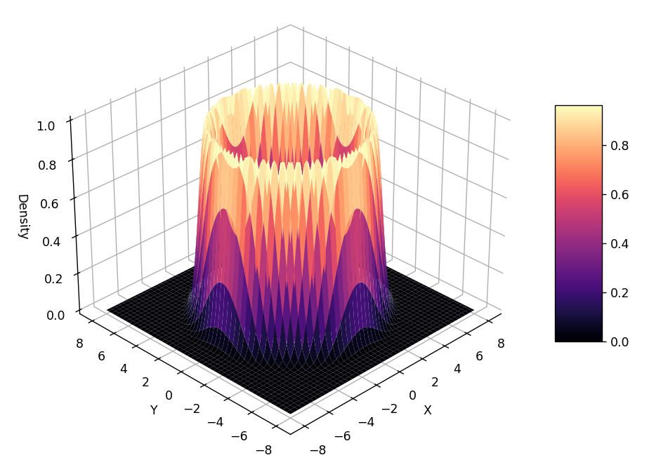
II. Estimating the ‘Volcano’ Distribution
Let’s attempt to pattern from a a lot much less ‘normal’ distribution that’s constructed in 2-dimensions, with the third dimension representing the distribution’s density.
Because the sampling is going on in (2D) house (the algorithm solely is aware of its x-y location not the ‘slope’ of the volcano) – we get a fairly ring across the mouth of the volcano.

Abstract of Mathematical Circumstances for MCMC
Now that we’ve seen the essential implementation right here’s a fast abstract of the mathematical situations an MCMC methodology requires to truly work:
| Situation | Mechanism |
|---|---|
| Stationary Distribution (That there exists a set of possibilities that, as soon as reached, won’t change.) |
Detailed Steadiness The algorithm is designed to fulfill the detailed steadiness equation. |
| Convergence (Guaranteeing that the chain ultimately converges to the stationary distribution.) |
Ergodicity The system should fulfill the situations in desk 2 be ergodic. |
| Uniqueness of Stationary Distribution (That there exists just one answer to the detailed steadiness equation) |
Ergodicity Assured if the system is ergodic. |
And right here’s how the MH algorithm satisfies the necessities for ergodicity:
| Situation | Mechanism |
|---|---|
| 1. Irreducible (Skill to succeed in any state from some other state.) |
Proposal Perform Usually glad through the use of a proposal (like a Gaussian) that has non-zero likelihood in all places. Word: If jumps to some areas are usually not potential, this situation fails. |
| 2. Aperiodic (The system doesn’t get trapped in a loop.) |
Rejection Step The “coin flip” permits us to reject a transfer and keep in the identical state, breaking any periodicity that will have occurred. |
| 3. Optimistic Recurrent (The anticipated return time to any state is finite.) |
Correct Likelihood Distribution Assured by the truth that we mannequin the goal as a correct distribution (i.e., it integrates/sums to (1)). |
Conclusion
On this article we’ve got seen how MCMC helps remedy the 2 predominant challenges of sampling from a distribution given solely its unnormalised density (chance) operate:
- The normalisation drawback: For a distribution to be a legitimate likelihood distribution the world beneath the curve should sum to (1). To do that we have to calculate the whole space beneath the curve after which divide our unnormalised values by that fixed. Calculating the world includes integrating a posh operate and within the case of the regular distribution for instance no closed-form answer exists.
- The inversion drawback: To generate a pattern we have to decide a random likelihood and ask what (x) worth corresponds to this space? To do that we not solely have to unravel the integral but additionally invert it. And since we are able to’t write down the integral it’s unattainable to unravel its inverse.
MCMC strategies, beginning with Metropolis-Hastings, enable us to bypass these unattainable math issues through the use of intelligent random walks and acceptance ratios.
For a extra sturdy implementation of the Metropolis-Hastings algorithm and an instance of sampling utilizing an uneven proposal (utilising the Hastings correction) take a look at the go code right here.
What’s Subsequent?
We’ve efficiently sampled from a posh (2D) distribution with out ever calculating an integral. Nonetheless, for those who have a look at the Metropolis-Hastings code, you’ll discover our proposal step is actually a blind, random guess (np.random.regular).
In low dimensions, guessing works. However within the high-dimensional areas of contemporary Bayesian strategies, guessing randomly is like making an attempt to get a greater fee from a usurer – nearly each proposal you make will likely be rejected.
In Half II, we are going to introduce Hamiltonian Monte Carlo (HMC), an algorithm that enables us to effectively discover high-dimensional house utilizing the geometry of the distribution to information our steps.


