Wall shear stress is the friction blood places on the wall of a vessel. It’s tied to the place plaque builds up, and it’s laborious to measure straight. What a clinic can get, with Doppler ultrasound for instance, is the rate at a couple of factors contained in the vessel. So the query for this text is whether or not a neural community can take these scattered, noisy velocities, along with the equations of fluid movement, and provides again the entire movement subject and the shear stress on the wall.
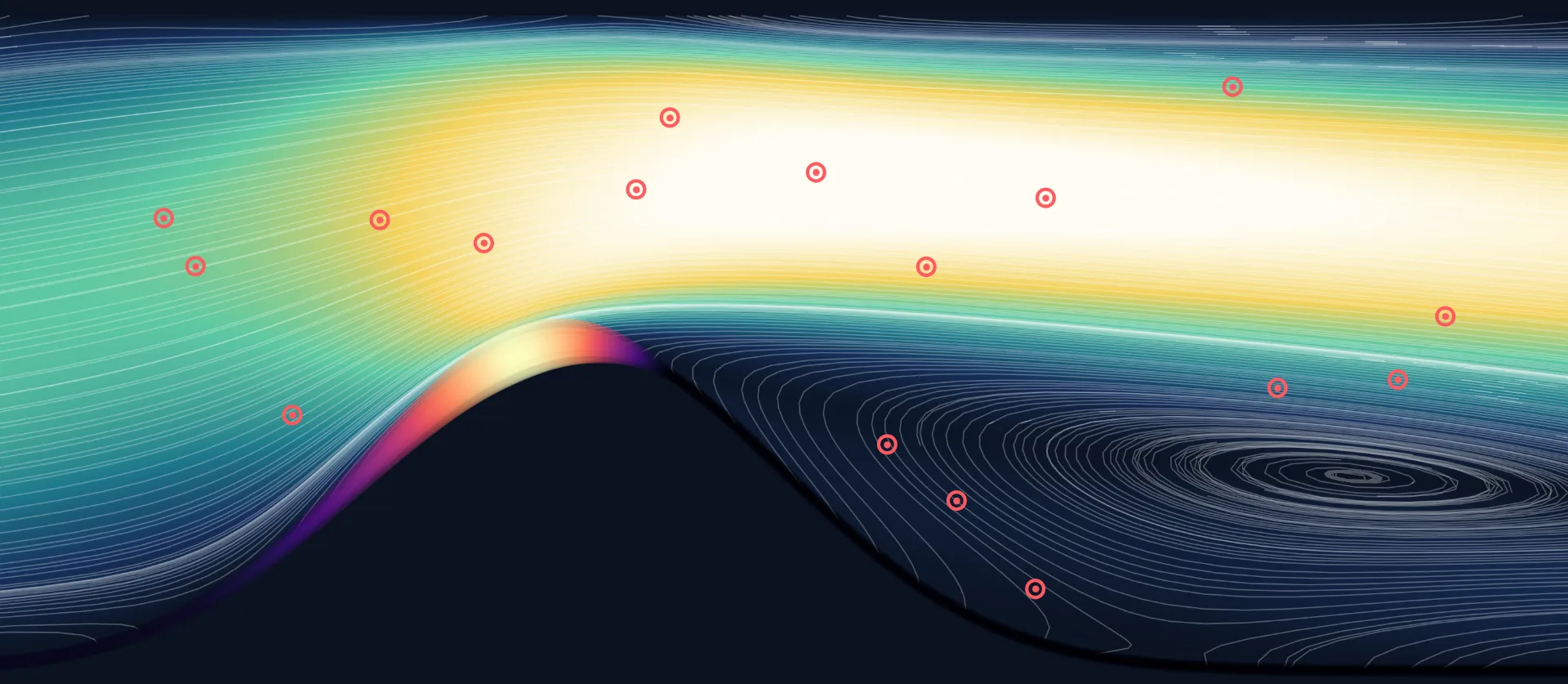
A physics-informed neural community (PINN) is a pure match. I constructed one in plain PyTorch, with out DeepXDE or some other PINN library, for a 2D artery with a narrowing (a stenosis). From 40 velocity readings it reconstructs the rate and stress fields and the area of reversed movement behind the narrowing. It additionally works out the viscosity of the fluid, which I handled as unknown, and its wall shear stress follows the CFD reference intently.
That is the primary article in a sequence about PINNs for blood movement. It covers the core: the Navier-Stokes residual, a learnable viscosity, and what decides whether or not the result’s any good. Later articles cowl the CFD solver behind the reference knowledge and a pulsating movement that follows a heartbeat.
The Setup
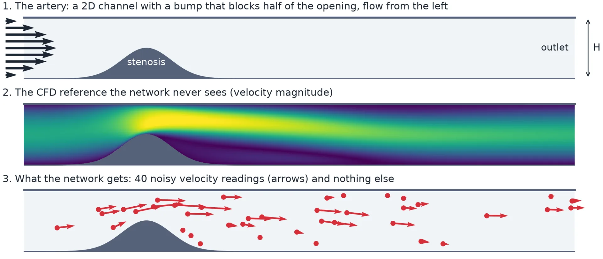
The artery is a 2D channel of peak H with a clean bump on the decrease wall that blocks half of the opening, a 50% stenosis. The movement is incompressible Navier-Stokes at a Reynolds variety of 200, with lengths measured in channel heights and velocities in inlet velocities. That may be a sluggish movement, on the low finish of what occurs in a carotid artery. In these items the kinematic viscosity is 0.005.
There aren’t any sufferers on this article, on function. To attain a reconstruction you’ll want to know the suitable reply, so I generated it. A Navier-Stokes solver I wrote (a projection technique on a staggered grid) computes the regular movement, and the PINN solely ever will get a couple of noisy readings taken from that answer. The noise is Gaussian, at 7% of the inlet velocity. I’d cowl the solver in a later article.
The size of the channel mattered greater than I anticipated. My first model was 5 heights lengthy. Behind the bump the movement separates from the wall and a area of reversed movement varieties. In 5 heights that area by no means closed: fluid was nonetheless transferring backwards on the outlet, the place the solver assumes it leaves. The outlet was shaping the reference answer as a lot because the physics was. Stretching the channel to 9 heights fastened it. The reversed movement now ends round x = 5.8 and every part after that runs ahead.
The readings are 40 factors contained in the fluid, every with a velocity vector plus noise. There aren’t any stress readings and no readings proper on the wall. I positioned them in 4 bands alongside the channel, with extra of them across the throat and the wake than close to the inlet and outlet. That format made little distinction, which I come again to on the finish.
The community is a plain MLP with 6 layers of 32 tanh items, about 5,500 weights. It makes use of tanh as a result of the momentum equation wants second derivatives of the output, and the second by-product of a ReLU is zero virtually all over the place. The inputs are rescaled to the vary -1 to 1 contained in the community, so autograd nonetheless differentiates with respect to the bodily coordinates.
Writing the Navier-Stokes residual in PyTorch
A PINN maps coordinates to bodily portions. Right here that’s (x, y) -> (u, v, p): two velocity elements and the stress. The loss has a time period that matches the measurements, like all regression, and a time period constructed from the residual of the equations: how badly the community’s personal output violates them. You get the residual by differentiating the community with respect to its inputs, which is what autograd is for. For incompressible Navier-Stokes there are three of them, continuity and one momentum equation per velocity part.
If these three are near zero at factors scattered over the channel, the community is near an answer of the equations, and the sensors select which one. The viscous time period wants u_xx, a by-product of a by-product, so autograd has to maintain the graph of the primary by-product round. That’s what create_graph=True does. Go away it out and the second name fails within the first epoch.
The loss provides up three teams, every with a weight:
-
knowledge, with weight 100, is the squared error towards the 40 readings -
pde, with weight 10, are the three residuals at 2,500 factors unfold over the fluid -
bc, with weight 10, no-slip on each partitions, are the inlet profile, and the outflow situation (zero stress and 0 streamwise gradient on the outlet)
The pde weight was the very first thing I bought flawed. At a weight of 1 the physics time period was too small to form something, and the rate error got here out greater than twice as giant as with 10. A weight of fifty did about the identical as 10. The collocation factors are resampled each 200 epochs, and 30% of them are picked the place the residual is at the moment largest. Coaching is Adam for 10,000 epochs with a decaying studying fee, adopted by 400 iterations of L-BFGS, which took round 35 minutes on three CPU threads.
Making viscosity a learnable parameter
In a ahead downside you realize all of the physics and need the sector. Right here the viscosity is unknown, so it turns into yet one more parameter, optimized alongside the community weights. It solely seems within the residual, because the quantity multiplying the second-derivative phrases. I retailer its logarithm, which retains it optimistic and places it on a scale the place an Adam step is cheap for a quantity as small as 0.005.
What do you begin it at? In apply you’d use a literature worth for blood, and that may be a wonderful start line. Right here I wished to examine that the reply comes from the sensors and never from the place the parameter started, so I began distant. One run began at 4 instances the true worth, one other at a couple of third of it. Each ended near the reality.
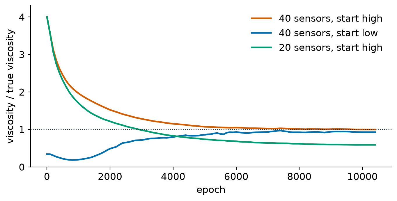
That final curve is the one to have a look at. Viscosity solely reaches the loss by the physics time period, and the physics time period solely means one thing as soon as the rate subject is roughly proper, so early in coaching the parameter strikes erratically and later it settles. What it settles on is determined by how a lot the info constrain the movement. With 20 sensors it went to the flawed worth each time I attempted, in each variant of the training fee and loss weights: between 1 / 4 and a half off, generally excessive and generally low, with loss curves that appeared wholesome the entire means. My studying is that twenty noisy factors can’t inform “thicker fluid, smoother movement” from “thinner fluid, sharper movement”, so the community picks certainly one of them.
With 40 sensors, and every part else the identical, viscosity landed on the suitable worth. Altering the training fee did far lower than including knowledge, which isn’t the reply I anticipated after I began tuning it.
Outcomes
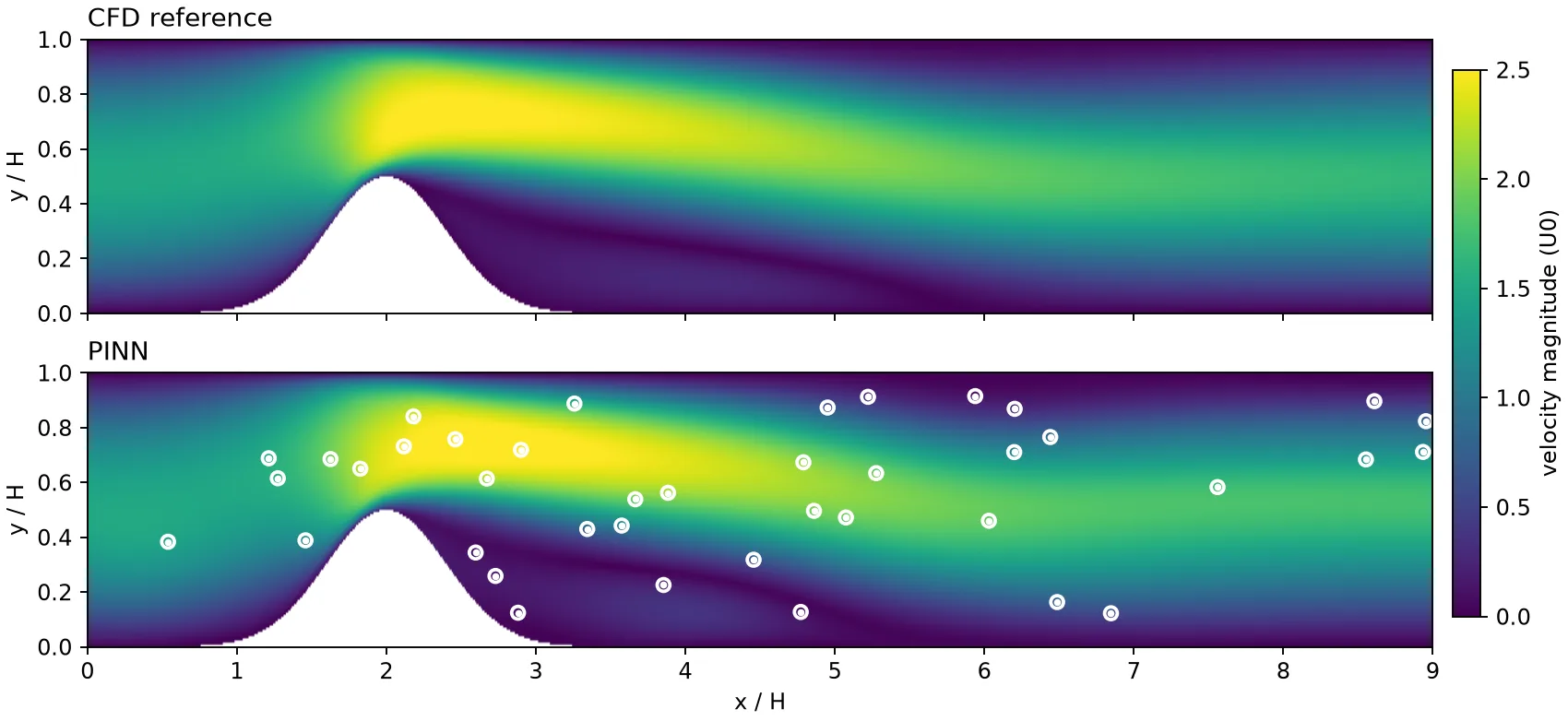
The reconstructed velocity subject is inside a couple of % of the CFD subject, about what I might count on from readings with this a lot noise in them. The v part alone appears worse in relative phrases, as a result of the movement is generally axial and the identical absolute error is split by a a lot smaller quantity.
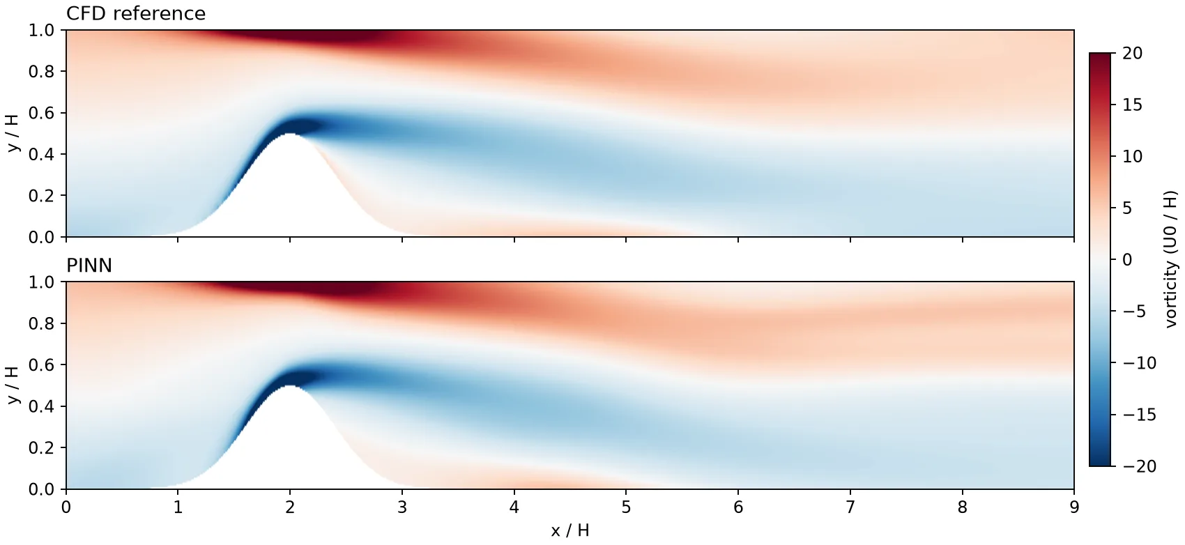
A velocity map can look proper whereas the movement construction is off, so I additionally in contrast vorticity, the native rotation of the fluid. The fascinating a part of this movement is the layer of sturdy shear between the quick jet and the sluggish reversed-flow zone, and the way it fades downstream.
The reversed-flow area is reproduced too. Within the CFD it begins at x = 2.2 and closes at about x = 5.75. Within the PINN it begins on the similar place and closes at about x = 5.6. No sensor sits on the wall, in order that comes from the physics working along with the readings.
The recovered viscosity on this run was 0.00498 towards a real 0.005, which is a little bit higher than typical. It was the primary run with 40 sensors. The opposite runs with 40 or extra sensors, with completely different beginning factors and completely different random attracts of the sensors, ended between 1% and eight% off.
For wall shear stress, which is what the train was for, the PINN’s curve follows the reference.
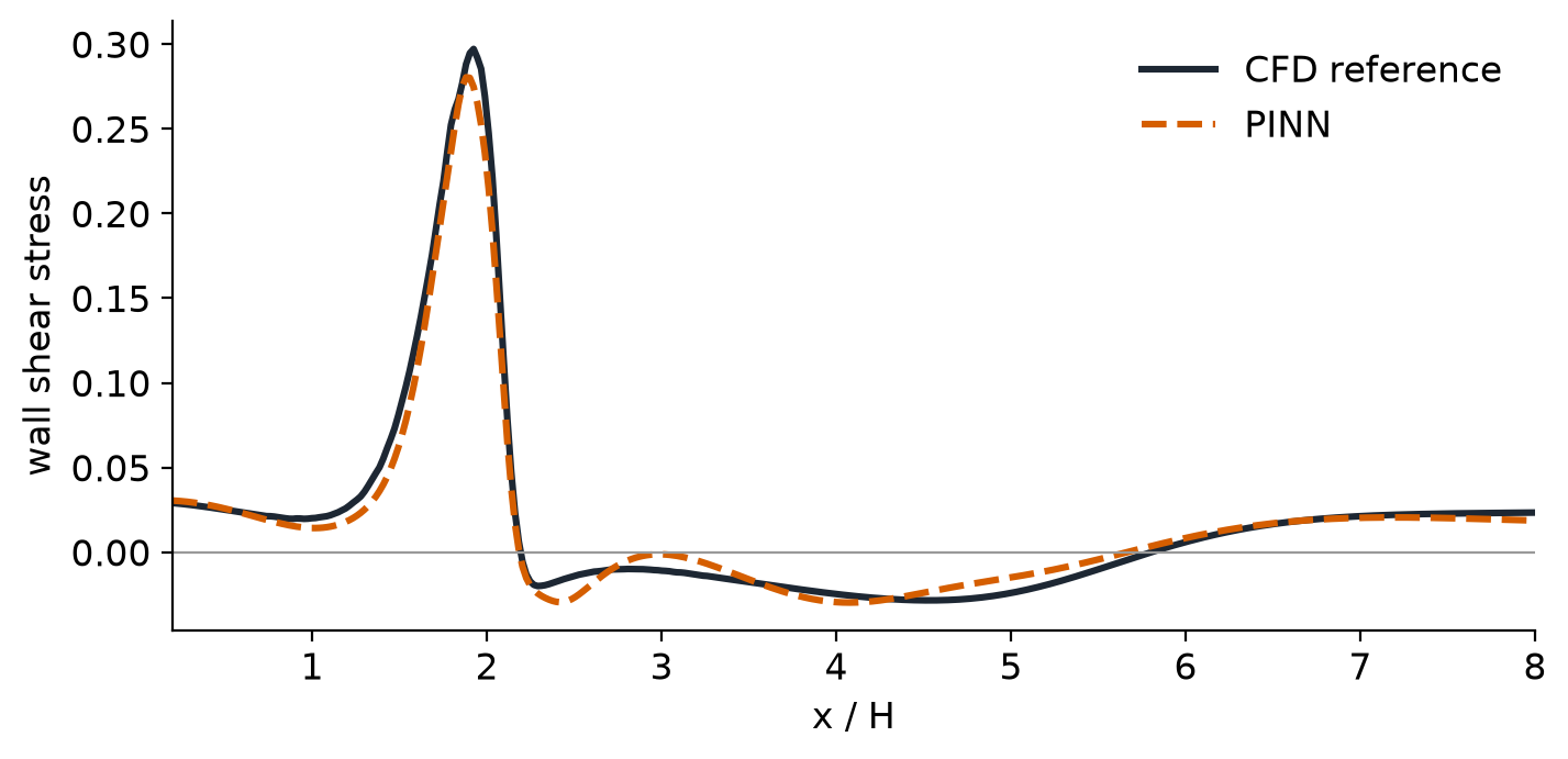
It has the suitable form all over the place, and its peak comes out a little bit low. One word on the reference. The solver’s staircase-shaped wall makes a uncooked finite-difference estimate of the wall gradient jagged. For each the CFD subject and the community I as a substitute take the rate alongside the wall regular at a couple of factors a brief distance from the wall and match the gradient by them, utilizing the truth that the rate is zero on the wall. Each curves are learn the identical means.
What made the distinction
Because the sensors mattered most, here’s what I different across the 40-sensor run. All of those used the identical community and coaching.
|
Change |
Impact |
|---|---|
|
20 sensors as a substitute of 40 |
viscosity 1 / 4 to a half off; velocity error the identical or worse |
|
60 sensors |
about the identical as 40 |
|
40 sensors unfold uniformly, not in bands |
barely worse vorticity, viscosity inside about 8% |
|
no outflow situation |
about the identical |
|
wider community (4 layers of 96) |
no higher, about twice as sluggish |
|
|
velocity error greater than twice as giant |
Scaling the inputs, decaying the training fee and choosing collocation factors by residual made little distinction to the rate error after I tried them on the primary channel. I stored them as a result of they value virtually nothing. The outflow situation modified little, so should you would moderately not inform the community about your outlet, you may depart it out right here.
Many of the enchancment got here from the info: sufficient sensors to pin the viscosity down, and a channel lengthy sufficient that the outlet stayed out of the best way. The structure and optimizer settings I attempted moved issues a lot much less.
The place this stops
The movement is 2D and regular, the partitions are inflexible, and the noise is obvious Gaussian noise, which stands in for a Doppler measurement with out modeling beam angle or speckle. Forty probes positioned wherever I selected can also be a beneficiant setup in contrast with an actual examination. The outcomes come from one geometry at one Reynolds quantity.
Blood can also be shear-thinning, so a continuing viscosity is least correct within the sluggish, separated zone behind the stenosis, proper the place the reversed movement sits. And the hyperlink between wall shear stress and plaque, whereas effectively studied, remains to be argued about.
The following article is in regards to the CFD solver that produced the reference knowledge, together with a bug in my wall-shear-stress reference that made a very good end result look dangerous. All code, configs and figures are within the repo: [link].