Guided Merge Type : An Optimized Sorting that Picks the Greatest from Bizarre and Multi-Manner Merge Type Algorithms

Introduction

On this article, I’m going to current a novel method for merging a number of sorted sequences into one referred to as guided Ok-merge and, based mostly on that, a general-purpose sorting algorithm referred to as guided Ok-merge type.

The present approaches to environment friendly merging of a number of sorted sequences require some helper information buildings, equivalent to a sorted array or a precedence queue. In distinction, guided Ok-merge retains the required data with the assistance of a number of isomorphic code fragments, and makes use of the goto operator to leap between them.

Theoretical analysis exhibits that guided Ok-merge reduces the time for such a multi-way merge, in comparison with the present implementation that makes use of a sorted array. On the identical time, guided Ok-merge doesn’t introduce any overhead, in distinction to the present implementation that makes use of a precedence queue.

Primarily based on all that, the sensible analysis exhibits that relying on the kind of information being sorted, guided Ok-merge type can carry out as much as 15% sooner, in comparison with the extensively used merge type algorithm.

This text is organized as follows:

···

1. Recalling merge, merge type, and Ok-merge type algorithms

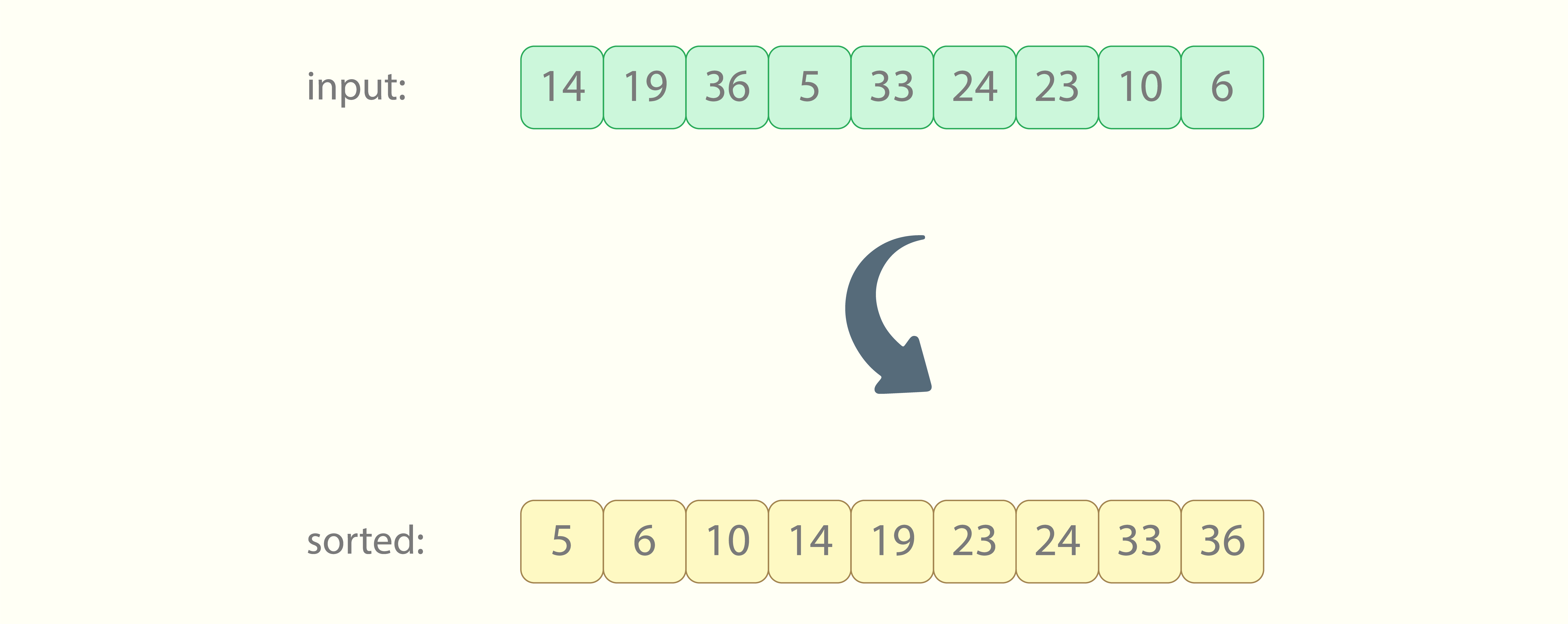
Sorting a sequence of values is a necessary process in Laptop science. Given an arbitrary sequence, after operating any sorting algorithm on it, we count on all its values to be rearranged – more often than not in rising order:

The need to type arises, for instance, when we have to:

• effectively navigate over giant volumes of knowledge, and discover needed gadgets there;

• current current information to the end-users in a clearer manner;

• determine sure patterns in giant volumes of knowledge;

• … and in lots of different instances arising in several fields.

There are completely different sorting algorithms, most well-known of that are in all probability bubble type, fast type, and merge type, every having its comparatively robust and weak sides.

Merge type (or some variation of it) is usually the default sorting algorithm in normal libraries of assorted programming languages. For instance:

• Java makes use of merge type when sorting an array of non-primitive information varieties,

• Python makes use of Timsort, which is a mix of merge type and insertion type algorithms,

• C++ makes use of merge type (or some variation of it) when the sorting have to be secure.

Recalling the merge type algorithm

Understanding the merge process and merge type algorithm is necessary for continuing with this text. There are numerous good tutorials and movies on the Internet, equivalent to [1], [2] and [3]. This sub-section may even assist recall them.

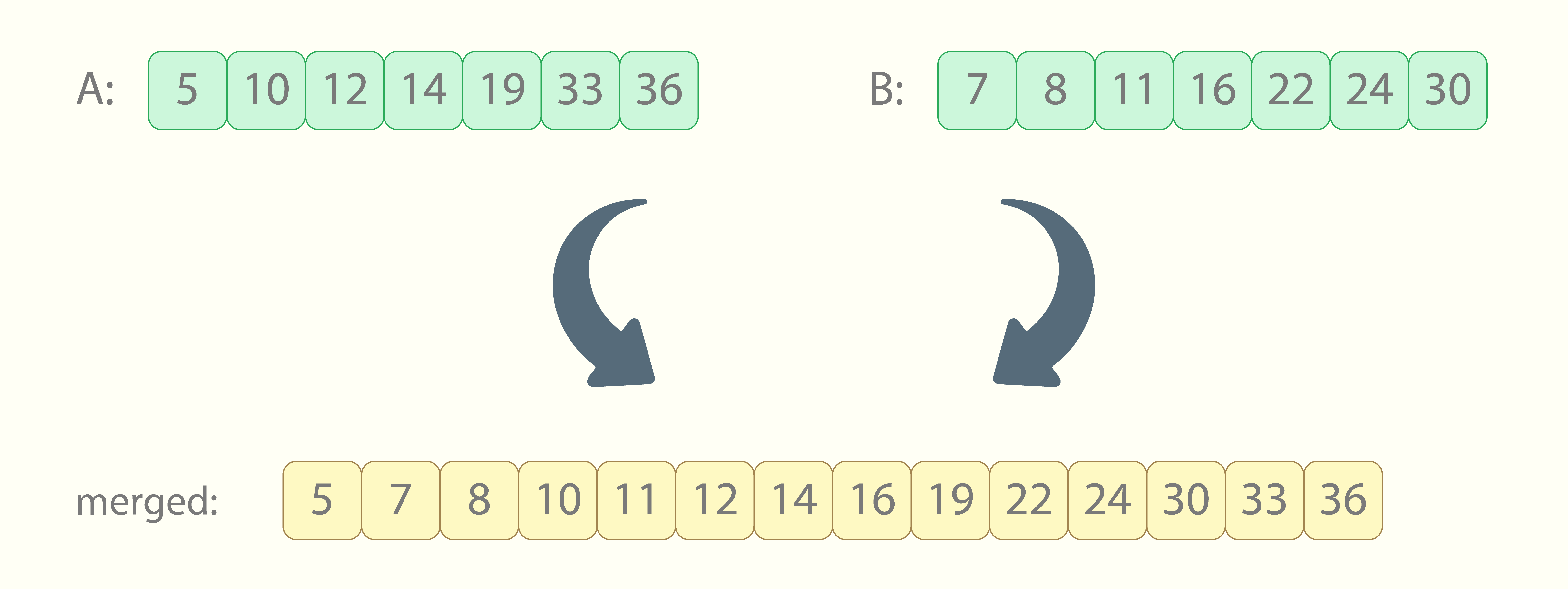
Merge type is a recursive algorithm, the constructing block of which is the merge process. Given two already sorted sequences, the aim of merge is to mix them into one, preserving the sorted state within the outcome:

Inside the merge process, each enter sequences ‘A’ and ‘B’ arrive in sorted order. Which means that after the merge, values of ‘A’ will protect their relative order within the output sequence, in addition to values of ‘B’ will:

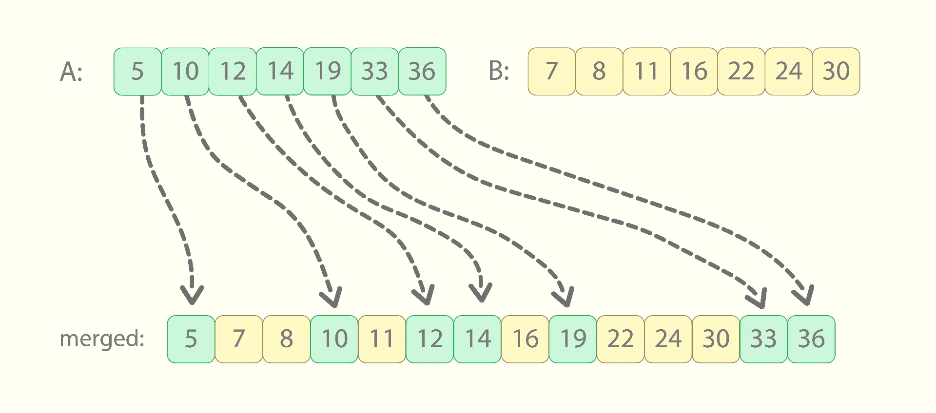
This truth permits us to provide the output sequence from left to proper, whereas scanning each enter sequences in parallel, additionally from left to proper.

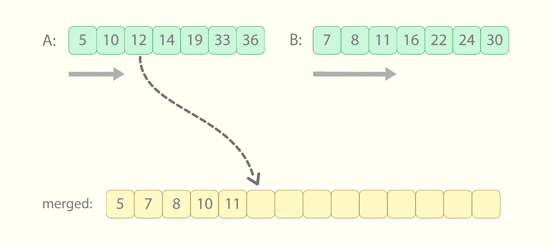
At each step, we’ll simply evaluate the following worth of ‘A’ with the following worth of ‘B’, and take the smaller one into ‘Out’.

Near the end, one of many sequences might be utterly moved to the output, whereas some brief fragment will stay within the different one. It means the values of the remaining fragment are larger than all of the values already thought of, so we will simply copy it to the output.

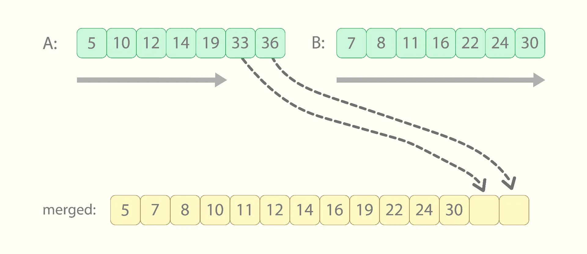
The code for the merge process in C++ turns into:

/// Merges two sorted arrays ‘A’ and ‘B’ into outcome array ‘Out’./// ‘n1’ and ‘n2’ are the lengths of arrays ‘A’ and ‘B’, respectively.void merge( const int A[], int n1, const int B[], int n2, int Out[] ) {	int i=0, j=0, m=0;  // Indexes over arrays ‘A’, ‘B’ and ‘Out’.	whereas ( i < n1 && j < n2 ) {  // We nonetheless have two arrays (tails) to merge		if ( A[i] < B[j] )			Out[m++] = A[i++];  // Subsequent worth of ‘A’ is appended to ‘Out’		else			Out[m++] = B[j++];  // Subsequent worth of ‘B’ is appended to ‘Out’	}	// One array is exhausted, so it stays     // to repeat the tail of the opposite array to ‘Out’	if ( i == n1 )		std::copy( B+j, B+n2, Out+m );  // Append the tail “B[j..n2)” to ‘Out’	else		std::copy( A+i, A+n1, Out+m );  // Append the tail “A[i..n1)” to ‘Out’}

The time complexity of merge is always O(n₁+n₂), where ‘n₁’ and ‘n₂’ are the lengths of the input sequences. That’s because all the “n₁+n₂” values need to be copied (or moved) to the output, and every copy is performed in a constant amount of time.

Now, the merge procedure outputs a sorted sequence, but it requires the input sequences to be sorted too. How can we use merge then to sort an arbitrary input array? The answer is: using recursion, and that is how the merge sort algorithm operates. What it does to sort an n-long input sequence is:

• divides it into 2 equal components (halves),

• recursively kinds every half, in an unbiased method,

• merges the sorted halves into the outcome array.

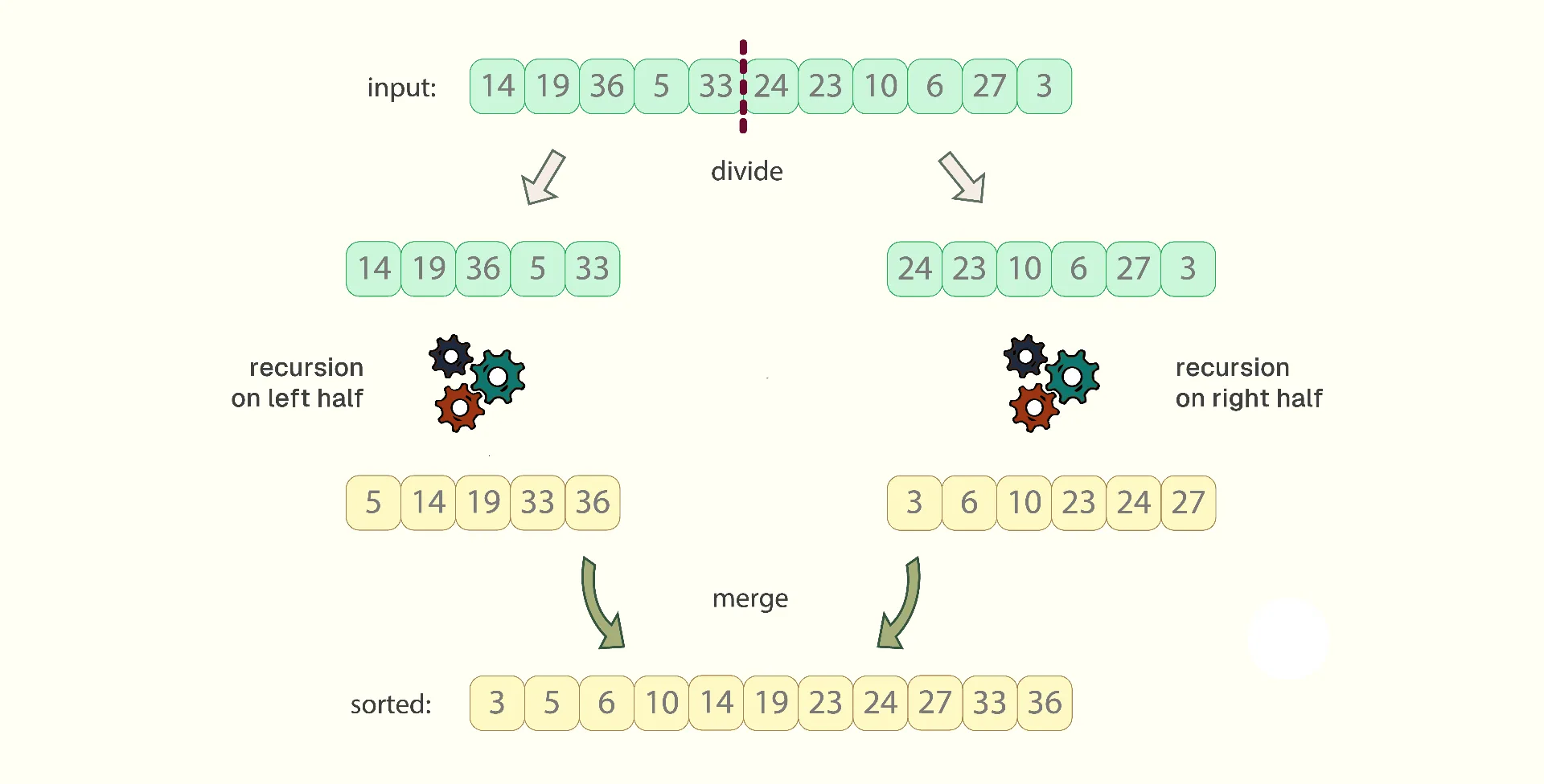
Which means that, when recursively sorting the left half, it is going to even be divided into 2 equal components (every being 1 / 4 now), every of which might be sorted recursively, earlier than being merged into the sorted left half. The identical additionally refers back to the proper half of the sequence.

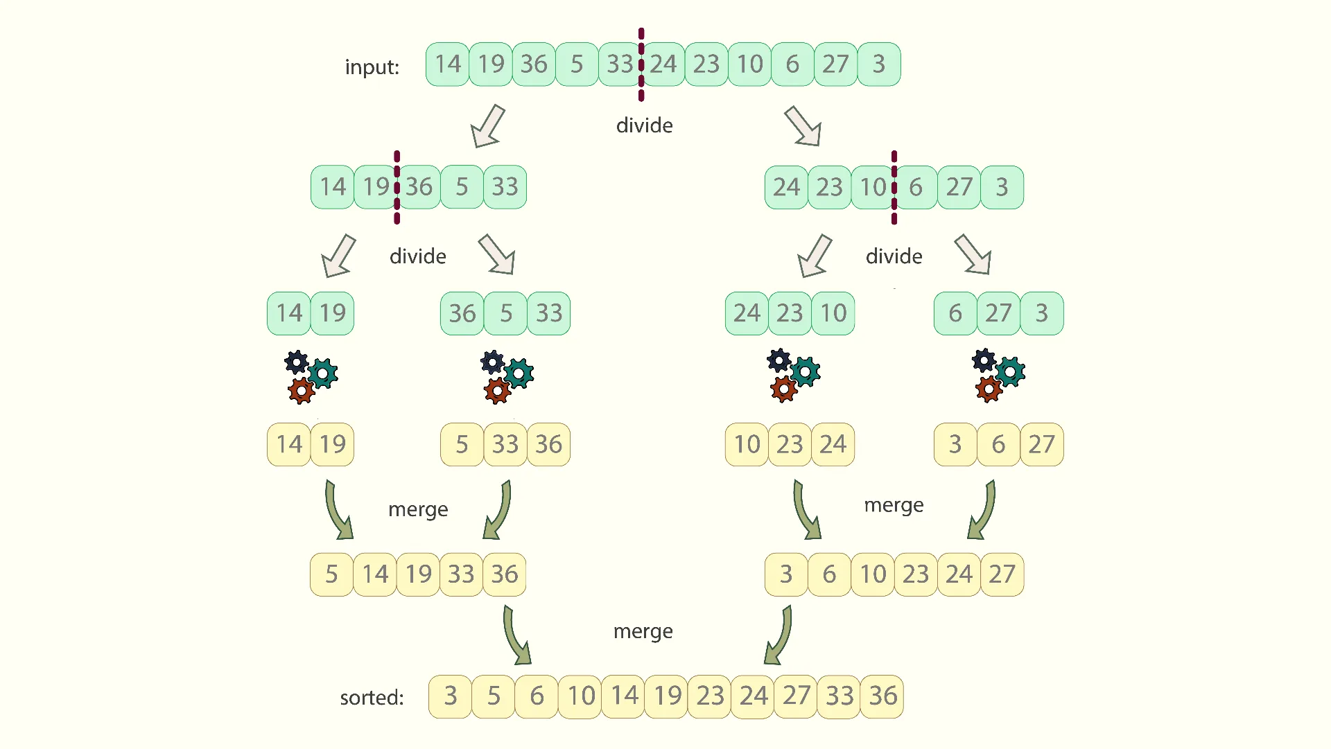
This manner, whereas recursion deepens, the present sub-array that must be sorted is shortened twice. The recursion stops when the algorithm reaches a 1-element sub-array, which, clearly, doesn’t require any sorting. Some optimizations cease recursion sooner, as soon as the present sub-array turns into shorter than a predefined threshold, after which they change to a less complicated sorting algorithm, usually to insertion type.

The code of the merge type algorithm in C++ turns into:

/// Kinds the n-long array ‘X’, in an rising order.void merge_sort( int X[], int n ) {	// Examine exit department first	if ( n < 16 ) {		// In keeping with a standard follow of assorted sorting 		// algorithms, right here additionally we change to Insertion type as soon as 		// the size of sub-array turns into sufficiently small.		insertion_sort( X, n );		return;	}	// In any other case, divide the n-long vary into 2 equal components	const int half = n / 2;	// Recursively type every half	//    Observe, due to the rounding in division by 2, the second 	//    half would possibly end in a shorter size.	merge_sort( X, half );	merge_sort( X+half, n-half );	// Quickly allocate a buffer for storing the results of the merge.	//    Observe, in an optimum implementation it is sensible to allocate 	//    buffer solely as soon as, and use it in each recursive name. We simply 	//    don’t try this right here for simplicity.	int* buffer = new int[ n ];	// Merge the two sorted arrays into one	merge( X, half, 			X+half, n-half, 			buffer );	// Copy again the merged sequence from buffer to authentic array	//   Observe, in an optimum implementation we should always use ping-pong 	//   merge type, thus merging the info to buffer on even ranges 	//   of recursion, and merging it again from buffer to ‘X’ on 	//   the odd ranges of recursion. That considerably reduces the 	//   time spent on copying-back from buffer. We simply don’t do it 	//   both, once more for simplicity.	std::copy_n( buffer, n, X );	delete [] buffer;}

As we see, merge type makes use of a brief buffer to retailer the output of the merge process. That is required, as we will’t write the merged sequence into the identical reminiscence location from which we learn both of its enter sequences ‘A’ or ‘B’. That’s why, on each invocation of “merge_sort”, first we write the merged sequence into the short-term buffer, after which copy it again to the unique array ‘X’.

There may be an optimization referred to as ping-pong merge type, which, when utilized, eliminates such copying again nearly completely. It does that by repeatedly swapping the roles of ‘X’ and ‘buffer’. Briefly talking, on the even ranges of recursion it merges intermediate outcomes from ‘X’ to ‘buffer’, whereas on the odd ranges of recursion it merges them from ‘buffer’ again to ‘X’. Nevertheless, for simplicity, we don’t implement the ping-pong optimization on this paper.

Recalling the Ok-merge type algorithm

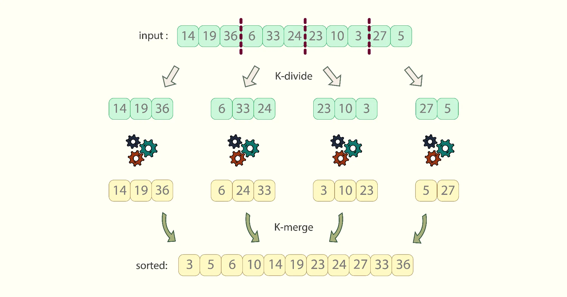
The algorithm that I’m going to explain is in truth an optimization of 1 variation of merge type, which known as Ok-merge type. The distinction between merge type and Ok-merge type is in what number of equal components the sequence is split into. If merge type at all times divides it into 2 components, then what Ok-merge type does is:

• divide the enter sequence into Ok equal components,

• recursively type them in an unbiased manner (making use of Ok-merge type to every of these components),

• mix the Ok sorted sequences into one, utilizing the Ok-merge process.

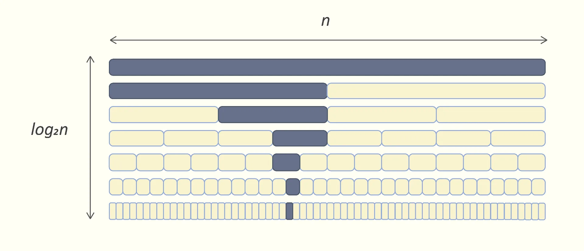
The benefit of Ok-merge type over extraordinary merge type is the lower in recursion depth. On each degree, merge type splits the present vary into halves, which, for an n-long enter sequence, requires “log₂n” ranges to succeed in the 1-long sub-range, thus, to succeed in the exit department of recursion:

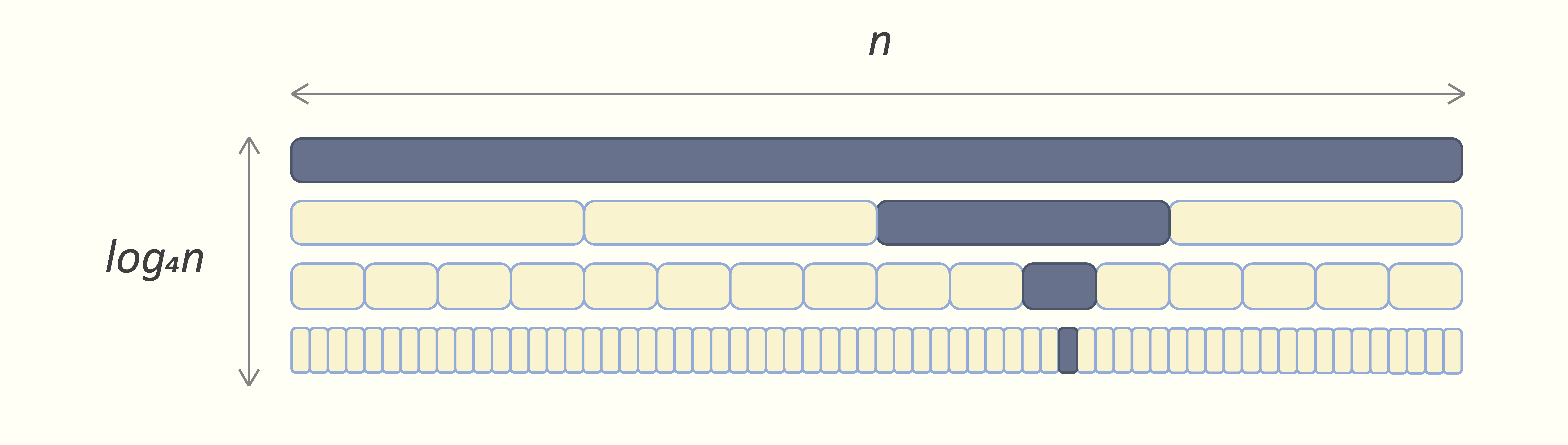
Whereas Ok-merge type at all times cuts the present vary into Ok equal components, it is going to require solely “log_Okn” ranges to carry the preliminary n-long enter sequence to 1-long ranges:

Inside Ok-merge type, because the depth of recursion decreases, so does the general variety of worth assignments. We will observe this with the assistance of the next diagrams: for extraordinary merge type, its full workflow will be depicted like this:

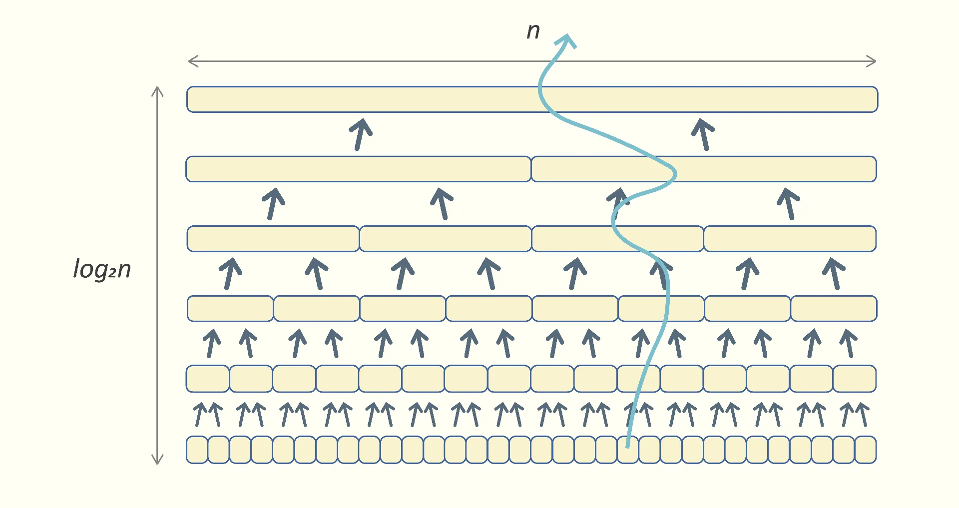
In keeping with the figurative arrows, the variety of instances each worth is assigned is proportional to “log₂n”. Thus, the variety of assignments throughout your entire algorithm turns into proportional to “n*log₂n”, which makes the time complexity of merge type O(n*log n).

For the Ok-merge type algorithm, the entire workspace turns into shorter:

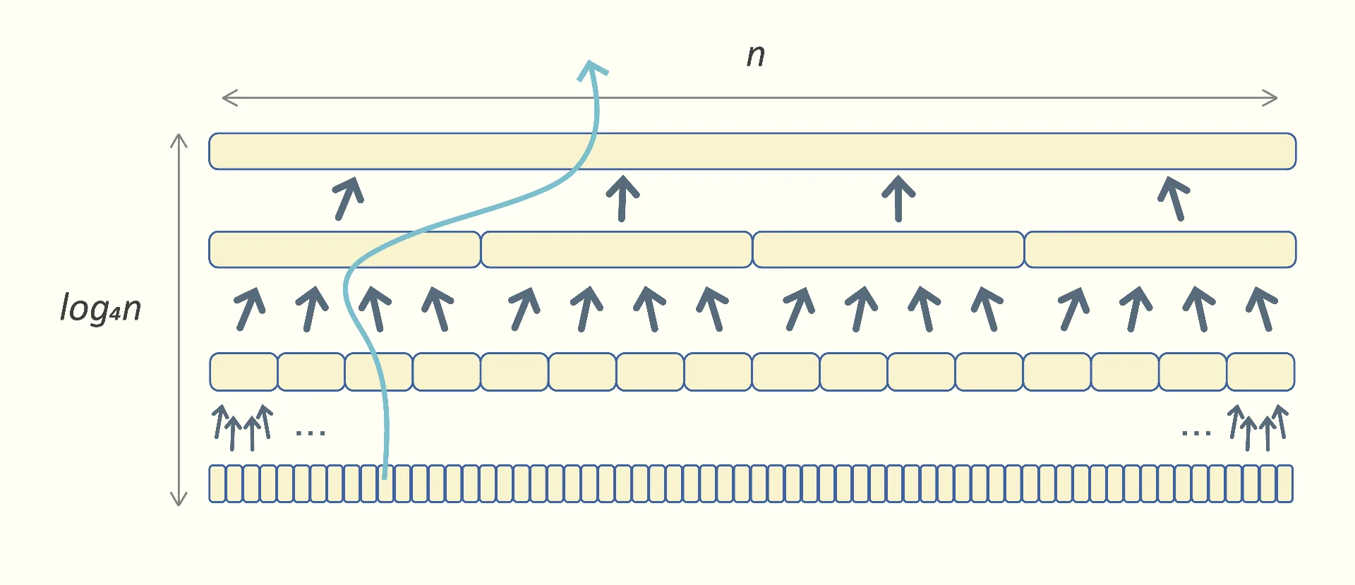
The variety of instances each worth is being assigned now’s proportional to “log_Okn”. Thus, the variety of assignments throughout your entire Ok-merge type turns into proportional to “n*log_Okn”.

We’d surprise why Ok-merge type isn’t the default sorting algorithm and isn’t extensively most well-liked over merge type.

The reply is that Ok-merge type has additionally one disadvantage: merging ‘Ok’ sorted arrays requires extra computation. When merging 2 arrays ‘A’ and ‘B’, at each step it is sufficient to evaluate the following worth of ‘A’ with the following worth of ‘B’, and duplicate the smaller one into the outcome. That’s why the code of the merge routine noticed earlier was that brief.

Whereas with regards to Ok-merge, so as to perceive which worth ought to go subsequent to the outcome array ‘Out’, we should always do extra comparisons. Let’s assume “Ok=4”, so we’re doing “4-merge”. To choose the smallest worth from the following 4 enter ones – “A[i]”, “B[j]”, “C[k]”, and “D[l]”, we should always carry out 3 comparisons now (please do not confuse the lowercase ‘okay’, which is the index over array ‘C’, with the uppercase ‘Ok’, which is the variety of components the sequence is being break up into):

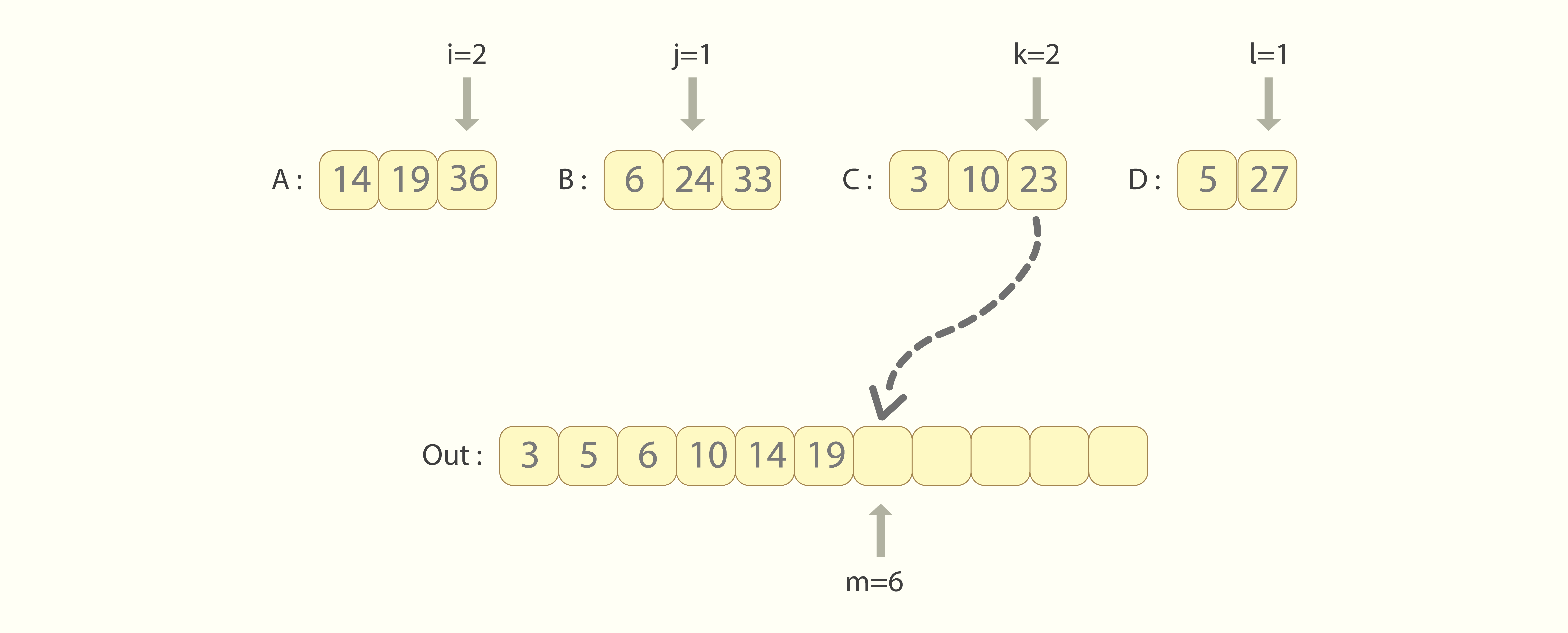
The code of the 4-merge process seems considerably longer:

/// Merges 4 sorted arrays ‘A’, ‘B’, ‘C’ and ‘D’ into outcome array ‘Out’./// ‘n1’, ‘n2’, ‘n3’ and ‘n4’ are the lengths of the enter arrays.void _4_merge( const int A[], int n1, const int B[], int n2, 		const int C[], int n3, const int D[], int n4, 		int Out[] ) {	int i=0, j=0, okay=0, l=0, m=0;  // Indexes over arrays ‘A’, ‘B’, ‘C’, ‘D’                                   // and ‘Out’.	whereas ( i < n1 && j < n2 && okay		// We nonetheless have 4 arrays (tails) to merge		if ( A[i] < B[j] ) {			// B[j] is actually not the smallest			if ( A[i] < C[k] ) {  // C[k] can also be not the smallest				// Stays to check ‘A[i]’ and ‘D[l]’				if ( A[i] < D[l] )					Out[m++] = A[i++];				else					Out[m++] = D[l++];			}			else {  // A[i] can also be not the smallest				// Stays to check ‘C[k]’ and ‘D[l]’				if ( C[k] < D[l] )					Out[m++] = C[k++];				else					Out[m++] = D[l++];			}		}		else {			// A[i] is actually not the smallest			if ( B[j] < C[k] ) {  // C[k] can also be not the smallest				// Stays to check ‘B[j]’ and ‘D[l]’				if ( B[j] < D[l] )					Out[m++] = B[j++];				else					Out[m++] = D[l++];			}			else {  // B[j] can also be not the smallest				// Stays to check ‘C[k]’ and ‘D[l]’				if ( C[k] < D[l] )					Out[m++] = C[k++];				else					Out[m++] = D[l++];			}		}	}	// One array is exhausted, so it stays to merge tails of the three others	if ( i == n1 )  // Array ‘A’ is exhausted		_3_merge( B+j, n2-j, C+okay, n3-k, D+l, n4-l, Out+m );	else if ( j == n2 )  // Array ‘B’ is exhausted		_3_merge( A+i, n1-i, C+okay, n3-k, D+l, n4-l, Out+m );	else if ( okay == n3 )  // Array ‘C’ is exhausted		_3_merge( A+i, n1-i, B+j, n2-j, D+l, n4-l, Out+m );	else  // ‘D’ is exhausted		_3_merge( A+i, n1-i, B+j, n2-j, C+okay, n3-k, Out+m );}

We see that together with the nested situations, at all times 3 comparisons are required to determine the smallest head worth between ‘A[i]’, ‘B[j]’, ‘C[k]’ and ‘D[l]’. Generalizing, at each step the Ok-merge type performs “Ok-1” comparisons to search out the smallest one from the ‘Ok’ present head values.

The price of doing extra comparisons compensates the benefit of creating fewer assignments. That’s the reason the less complicated merge type is most well-liked over Ok-merge type in follow. Nevertheless, Ok-merge type is perhaps most well-liked in different circumstances, for instance in exterior sorting (sorting exterior of the RAM), the place the price of evaluating 2 entries is far lower than the price of copying (or transferring) them.

Truly, there may be another method too for merging ‘Ok’ sorted arrays. There, all the present head values are saved in a specialised information construction, like a precedence queue, which permits quick retrieval of the smallest head worth in O(1) time, and its substitution with the following worth in O(log Ok) time. An in depth description of this method will be discovered at [4]. Nevertheless, utilizing such refined buildings at all times introduces important overhead. For instance, if the precedence queue is carried out as a binary heap, the overhead will come from:

• making swaps throughout sift–up and sift–down operations,

• checking to not transcend the bodily vary of the tree, and eventually,

• allocating needed house in dynamic reminiscence.

That’s the reason why a precedence queue is usually not used for merging just a few (“Ok=3” or “Ok=4”) sorted sequences, because the talked about overhead will definitely exceed attainable achieve in efficiency. Utilizing a precedence queue is justified when merging not less than dozens of sorted sequences.

···

2. The guided merge process

On this article, I’ll describe the guided merge type algorithm, which relies on the guided merge process. That is much like how extraordinary merge type relies on the merge process. So we’ll talk about guided merge first.

In truth, each guided merge and guided merge type ideas belong to the method the place we divide the present vary into ‘Ok’ equal components, not 2. So, to be extra exact, they need to be referred to as guided Ok-merge and guided Ok-merge type respectively. Nevertheless, generally I desire to omit the prefix “Ok” to make the naming extra compact and simply pronounceable.

On this chapter we’ll observe the case when “Ok=4”, so we might be merging 4 sorted enter sequences – “A”, “B”, “C” and “D”. As we already recalled, to try this Ok-merge algorithm repeatedly appears to be like for the following smallest worth between all the present heads (performing 3 comparisons per step), and appends it to the outcome sequence.

What if we act in another way? What if as an alternative of searching for the following smallest worth from scratch, we at all times preserve in reminiscence how the Ok present head values are ordered in relation to one another? In our instance, on the very first step, these 4 head values are “A[0]”, “B[0]”, “C[0]”, and “D[0]”, and their relative ordering is:

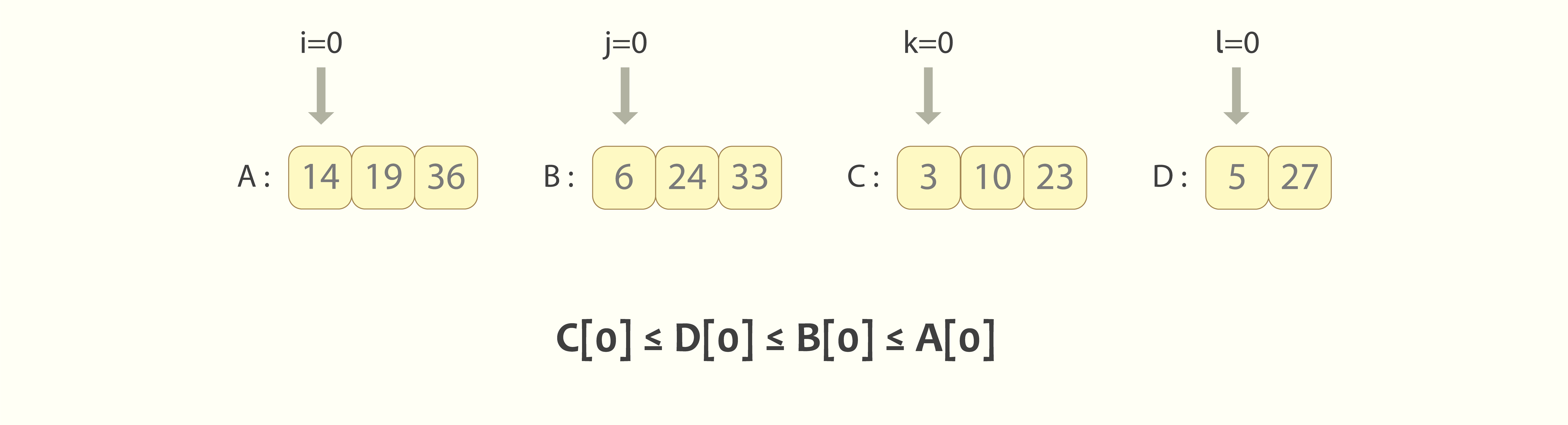
Having this, it’s simple that the preliminary smallest worth is the leftmost one amongst them – “C[0]”, and it must be taken to the outcome sequence first. Nevertheless, as soon as “C[0]” is there and “C[1]” involves substitute it through the subsequent choice to make, the opposite 3 values protect their relative order: “D[0] ≤ B[0] ≤ A[0]”, so “C[1]” will match someplace in between them or on the corners. The attainable preparations for “C[1]” are:

• “C[1] ≤ D[0] ≤ B[0] ≤ A[0]”, if the distinction “C[1] – C[0]” was sufficiently small, or

• “D[0] ≤ C[1] ≤ B[0] ≤ A[0]”, or

• “D[0] ≤ B[0] ≤ C[1] ≤ A[0]”, or, lastly

• “D[0] ≤ B[0] ≤ A[0] ≤ C[1]”, if the distinction “C[1] – C[0]” was giant sufficient.

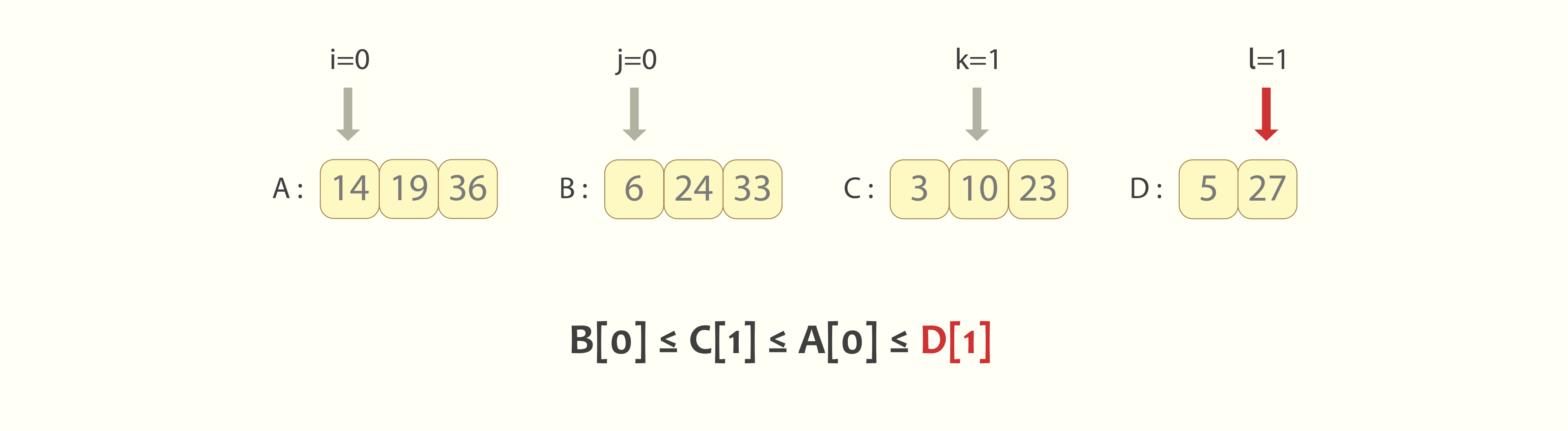
So what we have to perceive is: the place precisely the following head worth “C[1]” must be positioned within the remaining sorted checklist “D[0] ≤ B[0] ≤ A[0]” to maintain its sorted order. To determine that out, we’ll do a binary seek for “C[1]” there. That’s the key level of the guided merge algorithm. So, at first we’ll evaluate “C[1]” with the center worth of the sorted checklist: “B[0]”, and based mostly on the outcome, subsequent we’ll evaluate “C[1]” both with “D[0]” or with “A[0]”.

In our instance, “C[1] > B[0]” and “C[1] < A[0]”, so the following sorted checklist of head values might be “D[0] ≤ B[0] ≤ C[1] ≤ A[0]”.

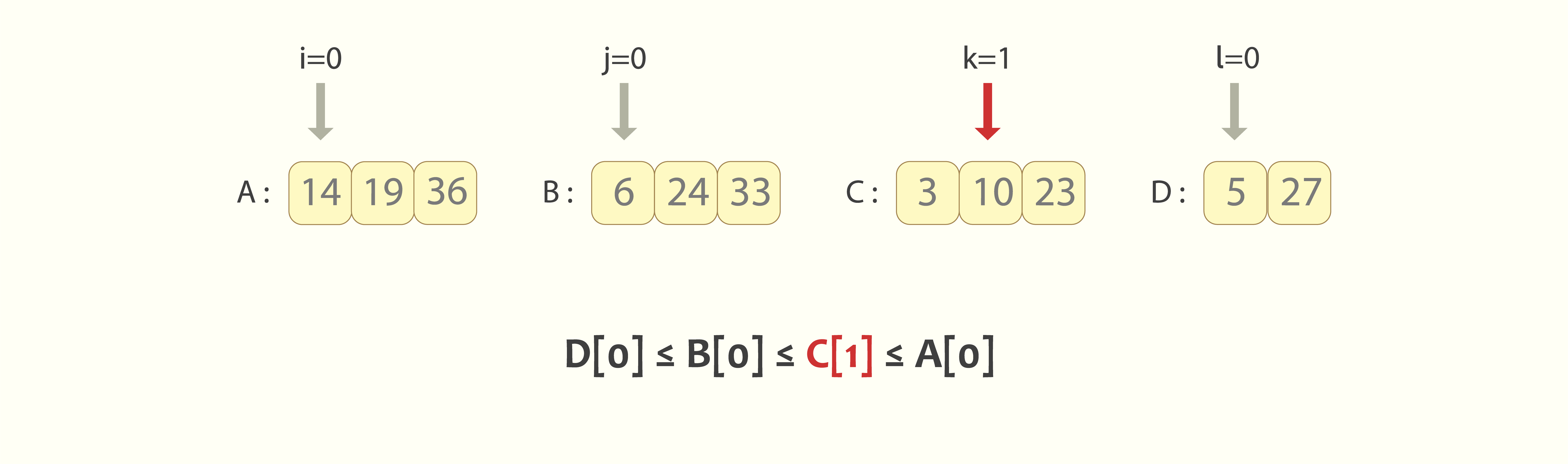
So we made solely 2 comparisons and discovered the following relative ordering of head values. This outperforms the Ok–merge algorithm, the place we had been doing “Ok-1=3” comparisons per step.

From this level, the algorithm repeats. Because the up to date relative ordering is “D[0] ≤ B[0] ≤ C[1] ≤ A[0]”, we’ll take the following smallest worth “D[0]” to the outcome sequence, and can correctly place its substitution “D[1]” into the remaining sorted checklist “B[0] ≤ C[1] ≤ A[0]”, to protect its sorted state. That may require simply one other 2 comparisons.

···

3. Implementation of guided merge process

The thought described above requires retaining monitor of the sorted checklist of present head values. For instance, in some unspecified time in the future in time it may be as:

C[k] ≤ D[l] ≤ B[j] ≤ A[i].

The simple manner to try this is to maintain a brief sorted array. Let’s title it “sorted_cursors”.

sorted_cursors[ 4 ] = [ (C[k], C), (D[l], D), (B[j], B), (A[i], A) ]

Observe that we might want to retailer not solely the top values themselves, but additionally references (or pointers) to the sequences from which these values had been taken. That is required so we’ll be capable of substitute, for instance, “C[k]” with “C[k+1]” on the following step, so we’ll know that the following head worth must be taken from the sequence “C”. As we already noticed within the earlier chapter, as soon as “C[k]” is positioned within the outcome and “C[k+1]” substitutes it, the following 4 attainable preparations of head values are:

• [ (C[k+1], C), (D[l], D), (B[j], B), (A[i], A) ] ,

• [ (D[l], D), (C[k+1], C), (B[j], B), (A[i], A) ] ,

• [ (D[l], D), (B[j], B), (C[k+1], C), (A[i], A) ] , and

• [ (D[l], D), (B[j], B), (A[i], A), (C[k+1], C) ] .

To effectively preserve such a “sorted_cursors” array, we should always left-shift a few of its values by one place and place the brand new pair “(C[k+1], C)” into the emptied slot:

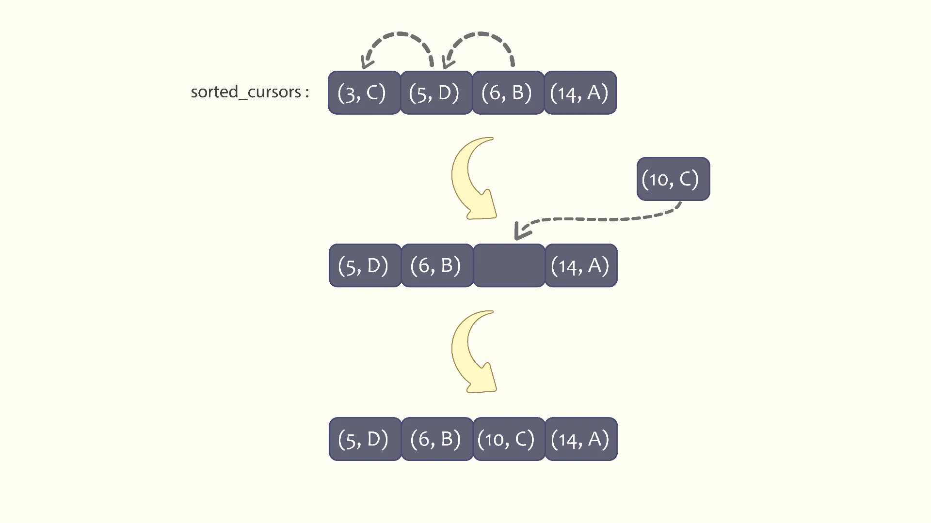
All that’s attainable and is, in truth, the simple approach to implement. However that’s not the perfect method for us, because it introduces a number of further assignments per step when doing the left-shifts.

As an alternative, the guided merge algorithm retains monitor of the present sorted sequence of head values by leaping between completely different fragments of the code. For a given ‘Ok’, there are “Ok!” attainable preparations of head values. In our case, as “Ok=4”, that’s “4! = 24” methods:

• “abcd”, (that means “A[i] ≤ B[j] ≤ C[k] ≤ D[l]”),

• “abdc”, (that means “A[i] ≤ B[j] ≤ D[l] ≤ C[k]”),

• “acbd”,

• “acdb”,

• “adbc”,

• …

• “dcab”,

• “dcba” (that means “D[l] ≤ C[k] ≤ B[j] ≤ A[i]”).

Ultimately, what I counsel is having a fraction of code for each attainable association. For the primary attainable association “abcd”, that fragment will appear like:

/// Performs guided merge of 4 enter arrays A[0..n1), B[0..n2), /// C[0..n3) and D[0..n4), writing the merged result into array “Out”.void guided_4_merge( const int A[], int n1, 		const int B[], int n2, 		const int C[], int n3, 		const int D[], int n4, 		int Out[] ) {	int i=0, j=0, okay=0, l=0;  // Indexes over the 4 enter sequences	int m=0;  // Index over the output sequence	// ...	// ...	// << preliminary choice of the case, that we are going to write a bit later >>	// ...	// ...abcd_label:  // At the moment “A[i] <= B[j] <= C[k] <= D[l]”	Out[m++] = A[i];  // Place the top of “A” into the outcome sequence	++i;  // Advance to the following worth “A[i+1]”	if ( i == n1 )  // Examine if sequence “A” is exhausted		goto finish_label;	// Carry out binary search of the brand new “A[i]” (previously “A[i+1]”) within the     // remaining sorted checklist “B[j] <= C[k] <= D[l]”	if ( A[i] <= C[k] ) {		if ( A[i] <= B[j] )			goto abcd_label;  // The ordering has not modified		else			goto bacd_label;  // The ordering is                               // “B[j] <= A[i] <= C[k] <= D[l]” now	}	else {		if ( A[i] <= D[l] )			goto bcad_label;  // The ordering turns into                               // “B[j] <= C[k] <= A[i] <= D[l]”		else			goto bcda_label;  // The ordering turns into                               // “B[j] <= C[k] <= D[l] <= A[i]”abdc_label:  // At the moment “A[i] <= B[j] <= D[l] <= C[k]”	// ...	// << comparable sequence of directions for the ordering “abdc” >>	// ...	// ...	// << comparable code fragments for the opposite 22 attainable preparations >>	// ...	// ...	// ...	// << finalization, which we'll write a bit later >>	// ...	// ...}

This manner, we could have 23 extra fragments, every corresponding to a different attainable association of the present head values “A[i]”, “B[j]”, “C[k]” and “D[l]”. Codes of all these fragments might be isomorphic, which is why in sure programming languages like C or C++, macros will be (and must be) used to keep away from duplication of supply code.

Having “Ok!” isomorphic code fragments, and utilizing the “goto” operator to leap between them compensates for the price of doing left-shifts and insertions into the brief array “sorted_cursors”. Observe that just one “goto” is sufficient, in comparison with a number of assignments through the left-shift. One other fascinating level is that the goto operator turns into irreplaceable if we need to act within the described manner.

The offered code additionally has “finish_label”, the place the execution jumps as soon as both of the 4 enter sequences is exhausted, and when it stays to merge the tails of the opposite 3 sequences. Then, as we desire to proceed with the guided merge logic, one other “3! = 6” labels should observe, every akin to a permutation of identifiers of three sequences. Absolutely, that’s preferable to implement as a separate perform, like “guided_3_merge”, which is why the ending of our perform “guided_4_merge” will appear like this:

void guided_4_merge( const int A[], int n1, 		const int B[], int n2, 		const int C[], int n3, 		const int D[], int n4, 		int Out[] ) {	int i=0, j=0, okay=0, l=0;  // Indexes over the 4 enter sequences	int m=0;  // Index over the output sequence	// ...	// ...	// << preliminary choice of the case, which we'll write a bit later >>	// ...	// ...	// ...	// ...	// << processing of the 24 completely different orderings of “A, B, C, D” comes right here >>	// ...	// ...finish_label:  // Right here solely 3 sequences stay to merge, and                // we should always verify which one was exhausted	if ( i == n1 )  // The primary sequence ‘A’ is exhausted		return guided_3_merge( B+j, n2-j, C+okay, n3-k, D+l, n4-l, Out+m );				// We merge remaining tails of ‘B’, ‘C’, and ‘D’, 				// which are actually ‘n2-j’, ‘n3-k’, and ‘n4-l’-long 				// respectively.	else if ( j == n2 )  // The second sequence ‘B’ is exhausted		return guided_3_merge( A+i, n1-i, C+okay, n3-k, D+l, n4-l, Out+m );	else if ( okay == n3 )  // The third sequence ‘C’ is exhausted		return guided_3_merge( A+i, n1-i, B+j, n2-j, D+l, n4-l, Out+m );	else // The fourth sequence ‘D’ is exhausted		return guided_3_merge( A+i, n1-i, B+j, n2-j, C+okay, n3-k, Out+m );}

Finalizing the code of “guided_4_merge“, earlier than the primary leap to one of many 24 completely different labels, we have to perceive which label will probably be. In different phrases, we have to work out the relative ordering of the preliminary head values A[0], B[0], C[0], and D[0]. That may be executed with handbook comparisons, like this:

void guided_4_merge( const int A[], int n1, 		const int B[], int n2, 		const int C[], int n3, 		const int D[], int n4, 		int Out[] ) {	int i=0, j=0, okay=0, l=0;  // Indexes over the 4 enter sequences	int m=0;  // Index over the output sequence	// Evaluating the 4 head values A[0], B[0], C[0] and D[0], to 	// work out the preliminary relative ordering, and leap proper there.	if ( A[0] < B[0] ) {		if ( B[0] < C[0] ) {			if ( C[0] < D[0] )				goto abcd_label;			else				...		}		else {			if ( B[0] < D[0] )				goto acbd_label;			else				...		}	}	else {		...	}	// ...	// ...	// << processing of the 24 completely different orderings of “A, B, C, D” comes right here >>	// ...	// ...	// ...	// ...	// << finalization, once we merge 3 remaining tails >>	// ...	// ...}

One other macro will be (and must be) used to keep away from inflation of the start a part of “guided_4_merge”. Observe that the preliminary choice of relative ordering is made solely as soon as.

The entire code for the guided merge procedures in C++, for the instances “Ok=3” and “Ok=4”, is obtainable on my GitHub at [5].

As we already famous, the offered method won’t be sensible for big values of ‘Ok’, as ‘Ok!’ will increase sooner than any exponent. However it’s utterly sensible when “Ok=3” or “Ok=4”, because the variety of attainable orderings is “3! = 6” and “4! = 24”, respectively. Observe that if “Ok=2”, the guided merge process downgrades to extraordinary merge.

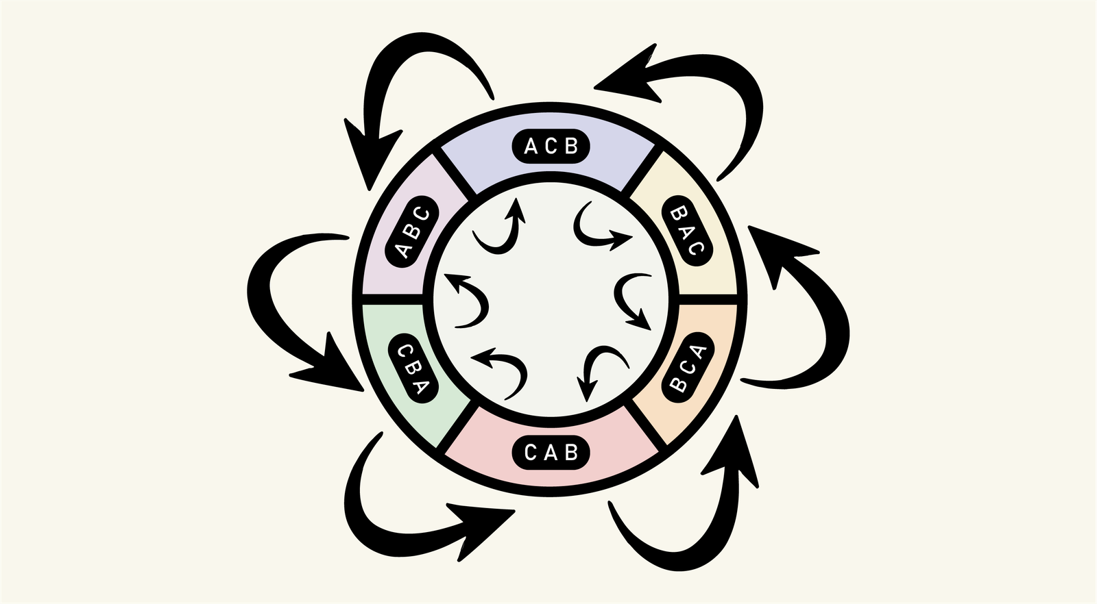
Earlier than ending this chapter, I need to add the diagram of attainable jumps over the “3! = 6” labels, for the case “Ok=3”:

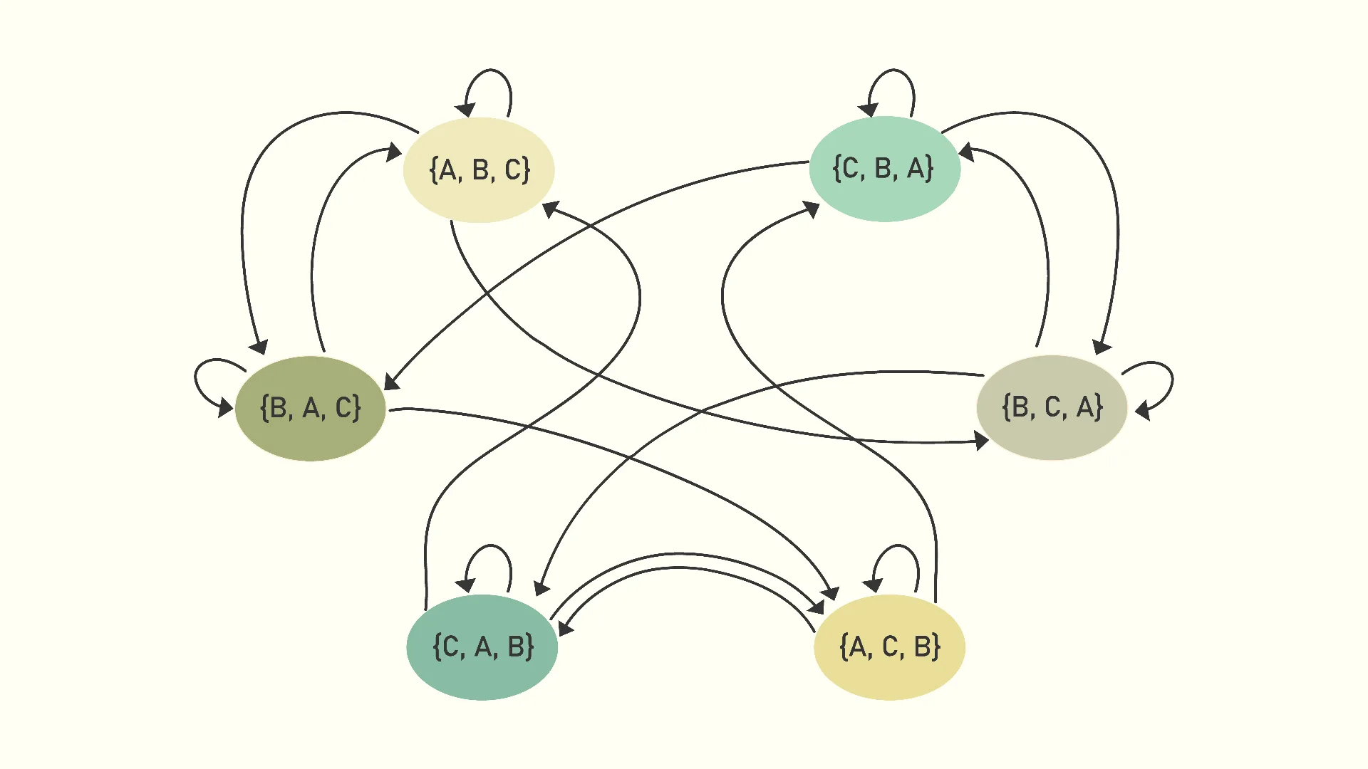
We see that, whereas on any label, solely 3 of the 6 labels can grow to be the following ones. For the case “Ok=4”, whereas on any label, solely 4 of the 24 labels can grow to be the following ones. That’s the reason we will count on a sensible benefit of guided Ok-merge over extraordinary Ok-merge.

I named the algorithm “guided merge” as a result of the impression is that we consistently information its execution over all attainable orderings of the ‘Ok’ head values. We’re at all times conscious not solely of the following smallest head worth, but additionally of their relative association.

···

4. The guided merge type algorithm

As soon as the guided Ok-merge process is derived, we will introduce guided merge type as a general-purpose sequence sorting algorithm. Guided merge type (or, extra exactly, guided Ok-merge type) is a recursive algorithm and depends on the guided merge (extra exactly, guided Ok-merge) process, precisely the identical manner that extraordinary merge type is a recursive algorithm and depends on the merge process.

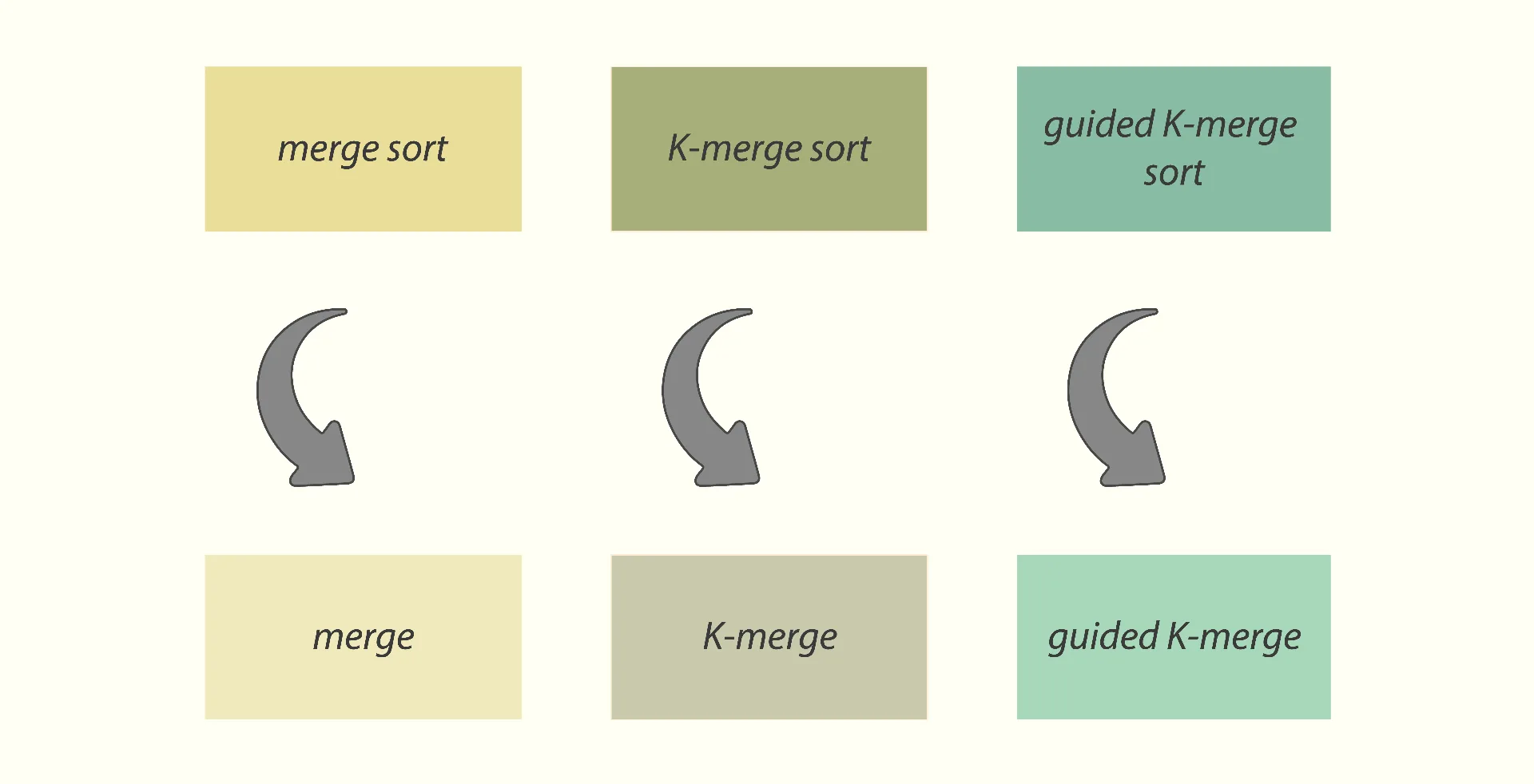
The logic of guided Ok-merge type is:

• divide the enter sequence into ‘Ok’ equal components,

• recursively type every of them by invoking the identical guided Ok-merge type algorithm,

• mix the outcome ‘Ok’ sorted sequences into one, utilizing the guided Ok-merge process.

We will already write the code of the guided Ok-merge type algorithm in C++:

/// Kinds the n-long array ‘X’, in an rising order.void guided_4_merge_sort( int X[], int n ) {	// Examine exit department at first, as this can be a recursive perform.	if ( n < 16 ) {		// In keeping with a standard follow of assorted sorting 		// algorithms, right here additionally we change to Insertion type when 		// the size of sub-array turns into sufficiently small.		insertion_sort( X, n );		return;	}	// In any other case, divide the n-long vary in 4 equal components	const int quarter = n / 4;	// Recursively type every half	//    Observe, due to the rounding in division by 4, the final half 	//    would possibly end in a shorter size.	guided_4_merge_sort( X, quarter );	guided_4_merge_sort( X+quarter, quarter );	guided_4_merge_sort( X+2*quarter, quarter );	guided_4_merge_sort( X+3*quarter, n-3*quarter );	// Quickly allocate a buffer for storing the results of the merge.	//    Observe, in an optimum implementation it is sensible to allocate 	//    buffer solely as soon as, and use it in each recursive name. We simply 	//    don’t try this right here for simplicity.	int* buffer = new int[ n ];	// Merge the 4 sorted arrays into one, utilizing “guided merge” algorithm	guided_4_merge( X, quarter, 			X+quarter, quarter, 			X+2*quarter, quarter, 			X+3*quarter, n-3*quarter, 			buffer );	// Copy again the merged sequence from buffer to authentic array	//   Observe, in an optimum implementation we should always use ping-pong 	//   merge type, thus merging the info to buffer on even ranges 	//   of recursion, and merging it again from buffer to ‘X’ on 	//   the odd ranges of recursion. That considerably reduces the 	//   time spent on copying-back from buffer. We simply don’t do it 	//   both, for simplicity functions.	std::copy_n( buffer, n, X );	delete [] buffer;}

As we see, the code is nearly similar to that of Ok-merge type. The one distinction is that as an alternative of “_4_merge”, the “guided_4_merge” process known as to mix the 4 sorted sub-arrays.

As guided Ok-merge type is a recursive algorithm that calls itself on shorter sub-arrays, within the first 10 strains there may be the exit department. As soon as the present sub-array turns into shorter than 16, we change to insertion type. This can be a widespread follow and is utilized in many different sorting algorithms, equivalent to introsort or timsort.

Subsequent, at strains 12-19 we divide the n-long enter sequence into 4 equal components. The final half would possibly outcome a bit shorter due to the rounding in integer division. Then, we recursively name guided_4_merge_sort on every of these components, and kind them independently from one another.

Lastly, at strains 20-39 we mix (i.e., merge) the 4 sorted arrays again into one, utilizing the “guided_4_merge” process. To not overcomplicate the code right here, first we merge them into a brief ‘buffer’, after which copy the outcome again to the enter array ‘X’. This copying again will be extremely optimized utilizing the ping-pong merge type method.

Additionally, in an optimized implementation, it is sensible to allocate the ‘buffer’ solely as soon as, and supply it to each name of “guided_4_merge_sort” as an additional argument. I simply determined not to try this both, to maintain the code right here so simple as attainable.

The time complexity of guided Ok-merge type is similar to that of Ok-merge type, and equals O(n log n).

The entire and extremely optimized implementation of guided Ok-merge type for the instances of “Ok=3” and “Ok=4” will be discovered on my GitHub at [5].

···

5. Theoretical analysis

On this chapter, we’ll do a theoretical comparability between guided Ok-merge type and Ok-merge type algorithms.

Because the logic of these two features is similar, if there are any causes for guided_k_merge_sort to outperform k_merge_sort, then these are the identical causes by which guided_k_merge outperforms k_merge. That is why we’ll focus solely on the latter comparability.

Analysis of Ok-merge

Assuming there are ‘Ok’ sorted sequences, k_merge repeatedly finds the following smallest head worth of them and locations it into the output sequence. So, if lengths of these sequences are:

n₁, n₂, …, n_Ok,

which in complete provides the size of:

n = n₁ + n₂ + … + n_Ok,

then precisely ‘n’ steps might be required to course of all of them, and duplicate (or transfer) every of their worth to the output.

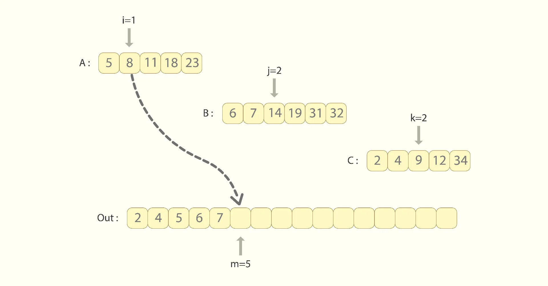
At each step, k_merge sequentially scans the present heads of all of the ‘Ok’ sequences, searching for the following smallest one. That requires ‘Ok-1’ comparisons. After the following smallest head is discovered, one task is completed to maneuver it to the output. So the variety of operations carried out throughout k_merge is:

“n*(Ok-1)” comparisons,
“n” assignments.

Right here we neglect the truth that in some instances, most values of some sequence(s) will be larger than all values of the opposite sequence(s). In such a case, the opposite sequences might be exhausted a lot sooner, leaving us with solely ‘Ok-1’ (and even fewer) sequences to merge, thus requiring fewer comparisons to be executed later. I suppose we will skip such eventualities right here, as a result of if there isn’t a dependency between values of the enter, their likelihood may be very small.

Analysis of guided Ok-merge

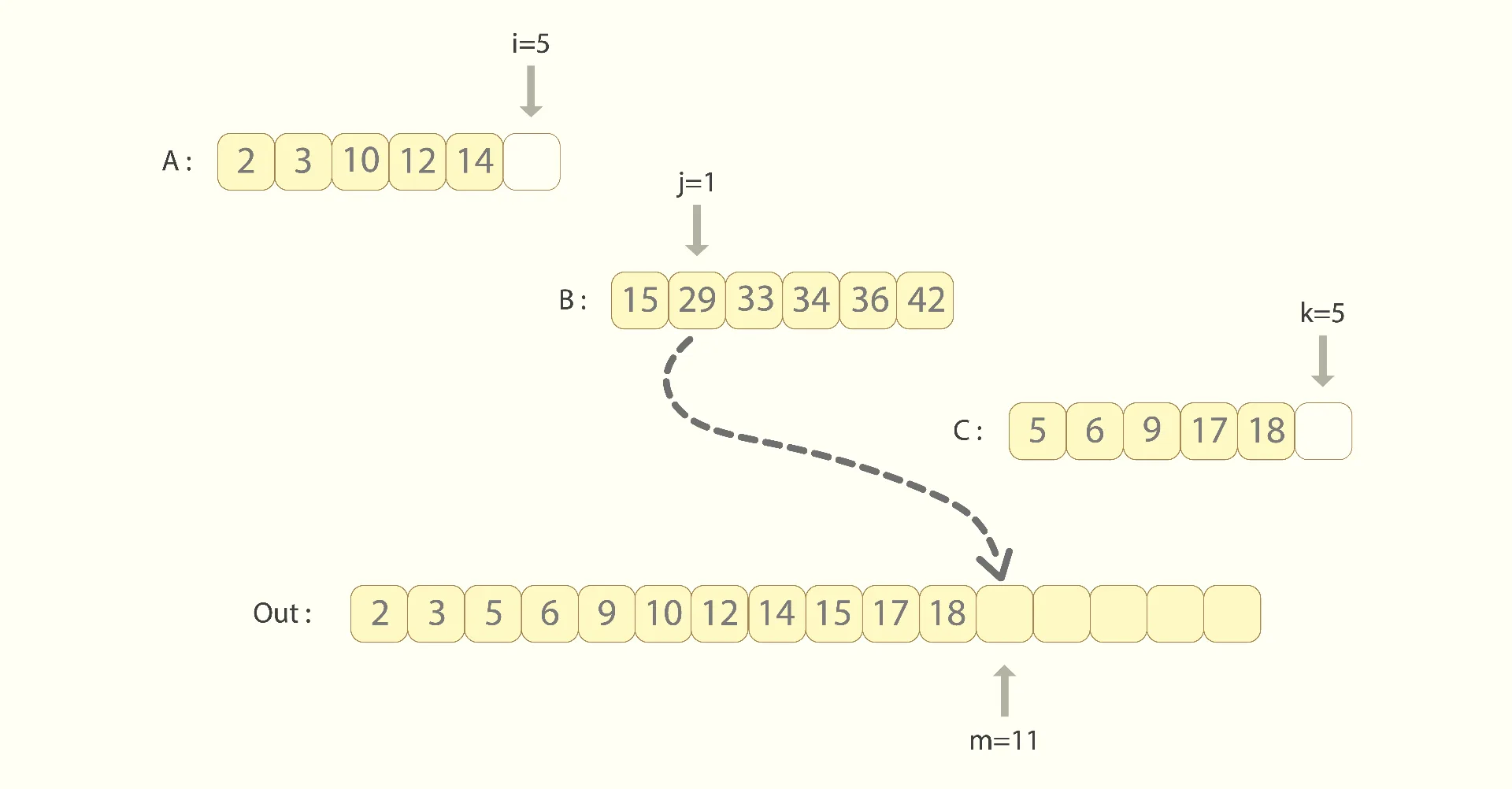
The end result of guided Ok-merge is similar to that of Ok-merge, as each algorithms copy (or transfer) all of the ‘n’ values to the output. So, in a basic case, guided Ok-merge additionally performs ‘n’ steps to make all these copies.

Nevertheless, guided Ok-merge additionally retains monitor of the relative order of the ‘Ok’ present head values.

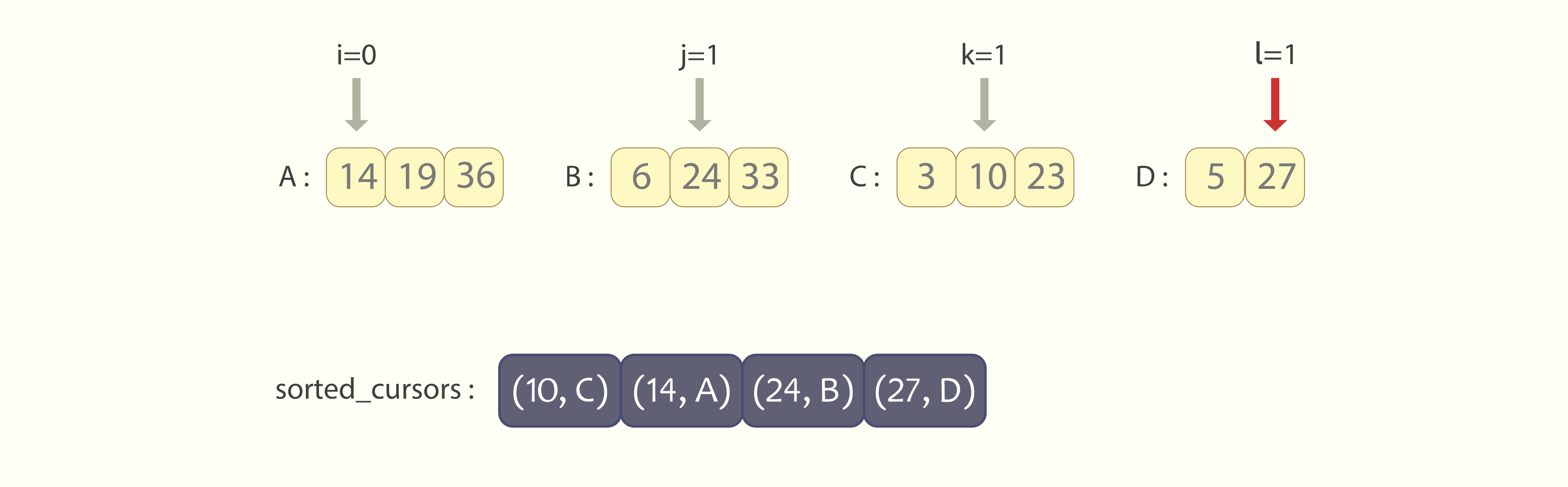
As we discovered within the earlier chapter, as an alternative of retaining the bodily array “sorted_cursors” in reminiscence, completely different preparations of its values will correspond to completely different sections within the code. Jumps between these sections are carried out with the goto operator.

Now what guided Ok-merge does on each step is:

• picks the following smallest head worth, as the primary one of many present association,

• locations it into the output [requires 1 assignment],

• substitutes it with the following worth from the identical sequence [requires a binary search in the “K-1”-long sorted list, thus, “log₂K” comparisons],

• jumps to presumably one other part, which corresponds to the following association of head values [requires one “goto” invocation].

Summarising, the general variety of operations carried out by guided Ok-merge is:

• “n*log₂Ok” comparisons,

• “n” assignments,

• “n” jumps.

As within the analysis of Ok-merge, right here we additionally neglect the likelihood that one of many ‘Ok’ enter sequences would possibly exhaust a lot sooner, leaving us with “Ok-1” (and even fewer) sequences to merge. If the enter values are distributed uniformly, the likelihood of such a situation may be very small.

We additionally neglect the price of determining the preliminary association of head values “A[0]”, “B[0]”, “C[0]”, …, as that’s carried out solely as soon as per guided Ok-merge.

Comparability between Ok-merge type and guided Ok-merge type

Evaluating Ok-merge and guided Ok-merge algorithms ends in the next desk:

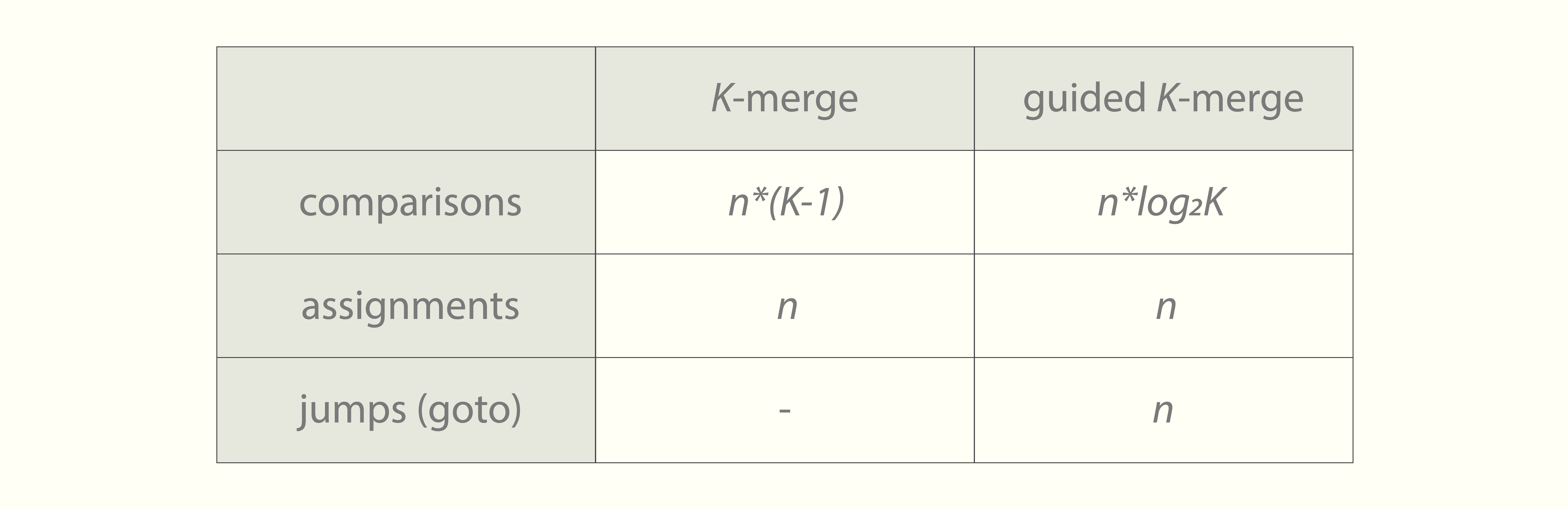
We see that guided Ok-merge performs fewer comparisons. That benefit turns into extra important as the worth of ‘Ok’ will increase. On the identical time, introducing too giant worth for ‘Ok’ will end in “Ok!” isomorphic fragments of code, which can each inflate the code dimension and nearly actually trigger cache misses when leaping between them; thus, will considerably enhance the runtime. Then again, introducing a really small worth for ‘Ok’, like “Ok=2”, will downgrade the guided Ok-merge algorithm into extraordinary merge.

Contemplating that the sorting algorithms are recursive with depth of “log_Okn”, the comparability between Ok-merge type and guided Ok-merge type ends in:

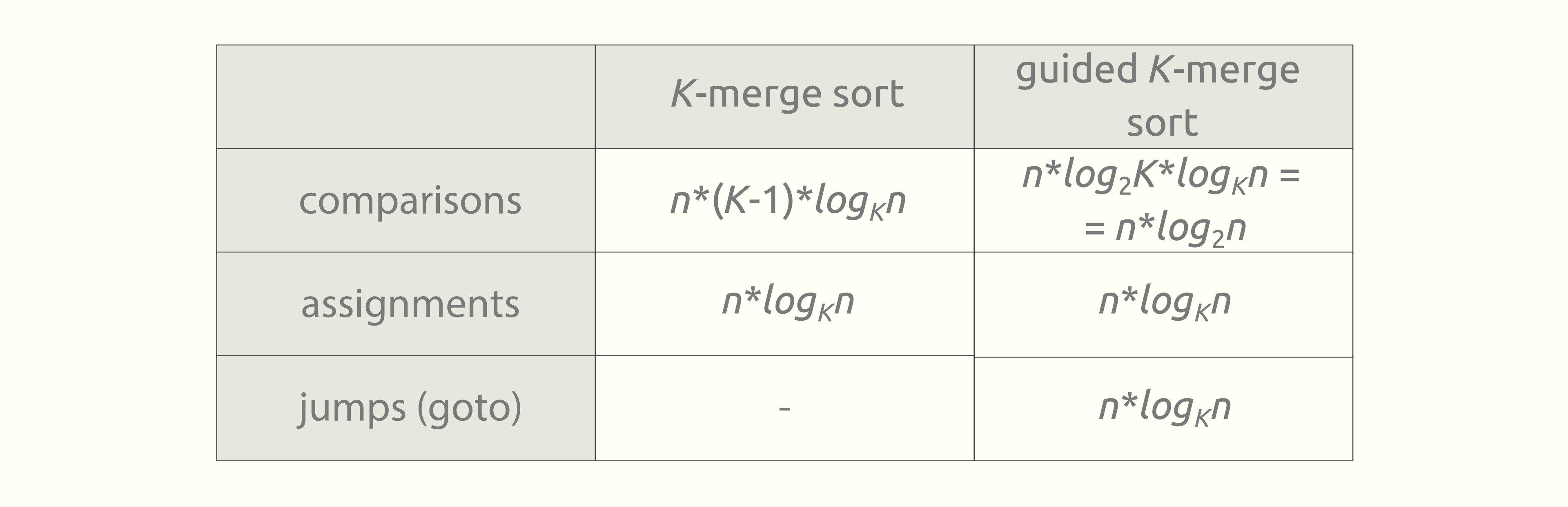
Within the subsequent part, we’ll experimentally work out the optimum worth of ‘Ok‘ to maintain the appropriate steadiness between the talked about elements.

···

6. Sensible analysis

On this chapter, we’ll observe outcomes of experimental comparability. The next sorting algorithms, all carried out in C++, had been benchmarked on randomly generated arrays:

• STL’s normal sorting routine – “std::type”,

• STL’s heap type – “std::make_heap”, adopted by “std::sort_heap”,

• extraordinary merge type,

• extraordinary merge type, that makes use of guided 2-merge underlying routine,

• 3-merge type,

• guided 3-merge type,

• 4-merge type,

• guided 4-merge type.

The experiments had been completely different from one another in:

• ‘n’ – size of the array being sorted,

• kinds of objects within the array,

• ‘switch_threshold’ – completely different thresholds for sub-array size, when over the past phases of recursion merge type implementations change to insertion type,

• arrays containing a lot of / few repeated values.

All of the experiments had been carried out beneath the next machine & surroundings:

• {Hardware}: Alienware m15 R6, eleventh Gen Intel® Core™ i7-11800H × 16, 16.0 GiB RAM

• Working system: Ubuntu 26.04 LTS, Linux 7.0.0-28-generic #28-Ubuntu SMP PREEMPT_DYNAMIC x86_64 GNU/Linux

• Compiler: g++ 15.2.0

• Compiler flags: -Wall -Wextra -std=c++17 -DNDEBUG -O3

• Benchmark library: Google Benchmark 1.9.1-1build1

All of the C++ code on which benchmarking was carried out will be discovered at [5].

Abstract of the outcomes

All experimental outcomes will be summarised within the following statements:

• The entire instances, STL heap type performs slower than std::type.

  • Rationalization: That is fairly anticipated, as std::type implements the introsort algorithm, which is a hybrid method that mixes fast type, heap type, and insertion type in the very best method.

• Bizarre merge type that depends on the guided 2-merge routine is a bit slower than the extraordinary merge type that depends on the usual merge routine.

  • Rationalization: An anticipated consequence, as a result of the code of the guided 2–merge process accommodates 2 goto directions, in distinction to the code of the usual merge process. Whereas theoretically each codes carry out precisely the identical actions, trendy CPUs are extremely optimised for parallelising and vectorising extraordinary loops, and never goto jumps.

• When sorting primitive information varieties (32-bit or 64-bit integers or floating-point numbers), std::type outperforms all different candidate algorithms, together with variants of guided merge type.

  • Rationalization: Repetitive comparisons and assignments of primitive variables are extremely optimised on trendy CPUs. Inside guided Ok-merge type, the price of jumps between code fragments in addition to the lack of the {hardware} to vectorise or parallelise such a code, surpasses its theoretical benefits of creating much less operations on primitive information varieties.

• When sorting giant objects (150-500 lengthy static or dynamic arrays of primitive information varieties), 3-merge type performs slower than extraordinary merge type, and 4-merge type performs even slower.

  • Rationalization: That is anticipated and will be noticed purely from theoretical analysis. With the expansion of ‘Ok’, the variety of comparisons grows linearly.

• When sorting the identical giant objects, guided 3-merge type outperforms each extraordinary merge type and std::type, whereas guided 4-merge type outperforms all of them much more.

  • Rationalization: That is the benefit of the guided Ok-merge type algorithm over others, together with extraordinary merge type, and even STL’s normal std::type. Such a outcome can also be anticipated from the theoretical analysis. Inside guided Ok-merge type, with the expansion of ‘Ok’, the variety of comparisons stays the identical – “n*log₂n”, whereas the variety of assignments drops, being equal to “n*log_Okn”. When sorting giant objects, the vast majority of the time goes on evaluating and assigning them to one another, so the time spent on jumps between code fragments, in addition to the lack of the CPU to vectorise operations, are compensated. That’s the reason on this situation, sensible analysis seems alike the theoretical analysis.

Benchmarking

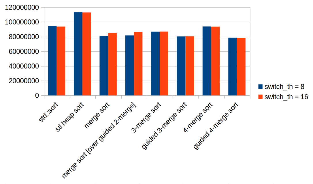
Listed here are the timings of sorting 150-long dynamic arrays of 64-bit integers. Size of the sequence being sorted is “n = 50’000”:

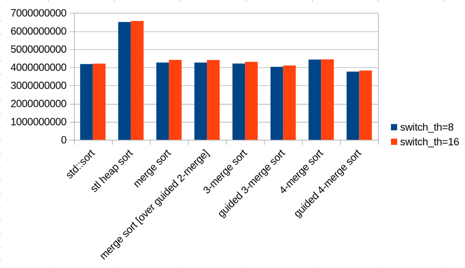
And listed below are the timings of sorting 250-long static arrays of 64-bit integers. The size of the sequence being sorted is “n = 750’000” now:

···

7. Conclusion

Within the present article, I’ve described the guided Ok-merge process and have derived the guided Ok-merge type general-purpose sorting algorithm.

The novelty right here is in how the ‘Ok’ sorted sequences are being merged into one. In distinction to extraordinary merge or Ok-merge procedures, guided Ok-merge doesn’t preserve any helper data in containers, and as an alternative makes use of “Ok!” isomorphic fragments of code, and jumps between them with the goto operator.

This effectively reduces the variety of operations carried out per step, making solely ”log₂Ok” comparisons, as an alternative of the “Ok-1” comparisons of the Ok-merge process.

The downside of guided Ok-merge is that “Ok!” isomorphic fragments seem within the code. So, to keep away from inflating the scale of this system, choosing values “Ok=3” or “Ok=4” guarantees the perfect steadiness between efficiency and the reminiscence used.

Implementation of the guided Ok-merge type algorithm in C++ for instances “Ok=3” and “Ok=4” will be discovered on my GitHub at [5].

For those who’ll have any strategies, questions, or will spot a mistake within the textual content, be happy to contact me by LinkedIn (the hyperlink beneath).

Thanks a lot for studying until the tip!

···

My gratitude to:

• Elen Grigoryan, for cautious design of all used illustrations (behance.internet/elengrigoryansun),

• Meri Movsesyan, for detailed evaluate of the article’s draft (linkedin.com/in/mermovs/).

For those who loved this text, be happy to contact me on LinkedIn (linkedin.com/in/tigran-hayrapetyan-cs/).

All the pictures had been designed upon request of the creator.

···

References

[1] – Sorting Algorithms, Half 1: Merge Type, by Vyacheslav Efimov: https://towardsdatascience.com/merge-sort-explained-and-visualised-660f6946d9b5/

[2] – Making Sense of Merge Type [Part 1], by Vaidehi Joshi: https://medium.com/basecs/making-sense-of-merge-sort-part-1-49649a143478

[3] – “Be taught Merge Type in 13 minutes”, by BroCode: https://www.youtube.com/watch?v=3j0SWDX4AtU

[4] – “Direct okay-way merge”: https://en.wikipedia.org/wiki/Ok-way_merge_algorithm#Direct_k-way_merge

[5] – Implementation and benchmarking of guided Ok-merge type in C++: https://github.com/tigranh/guided_merge_sort