The Most Stunning Statistic: The Historical past and the Science of the Humble Imply

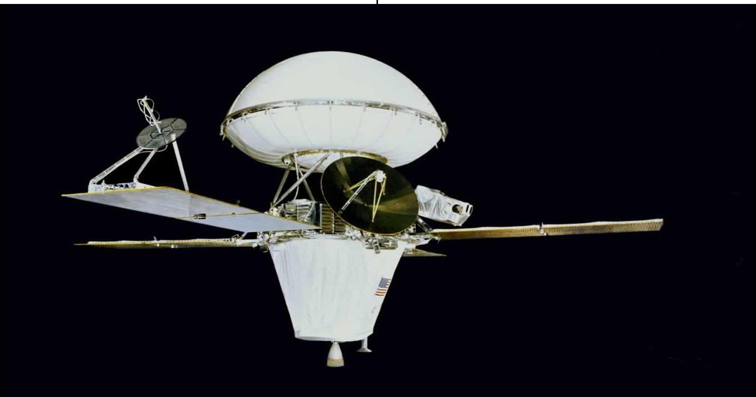
, 1976, the Viking 1 spacecraft entered Mars orbit.

A month later, as a midsummer night time stretched pleasantly forward of them in Pasadena, California, dozens of NASA controllers helplessly watched a feed delayed by 19 minutes because the Viking 1 lander separated from the orbiter.

Three hours later, the lander plunged into the Martian ambiance at 10,000 miles per hour. Ten minutes later, following a fiendishly complicated strategy, and with zero assist from JPL, the lander made an ideal landing on Mars.

For Mission Management, it hadn’t helped that, when Viking 1 entered Martian orbit and pointed its digital camera down on the floor, the initially chosen touchdown web site turned out to be “a minimum of twice as tough because the Mars common” prompting a frantic seek for a brand new web site.

Thankfully, a safer web site was discovered which, within the scientists’ phrases, was nonetheless “rougher than the Martian common,” however “close to the Martian common for elevations accessible to Viking” and “close to the Mars common in reflectivity.”

Even at 212 million miles from Earth, the standard imply turned out to be the statistical machine guiding Viking 1 to a protected spot in an unfriendly world.

The imply retains making its usefulness felt in all kinds of conditions, usually in really non-obvious methods. Take into account, for example, one other happenstance.

5 days after the Viking lander touched down on Mars, on July 25, 1976, the Viking orbiter transmitted to Earth, the next {photograph}.

The picture was instantly dismissed as a mere play of sunshine and shadow coupled with lacking knowledge (the darkish “speckles” within the picture). Nonetheless, it turned one of the crucial well-known examples of pareidolia: our tendency to detect patterns, particularly faces, and ascribe which means to them.

And it isn’t simply faces on Mars or the Moon.

Individuals have noticed animal shapes and UFOs amid clouds. Down on Earth, individuals have noticed cups and saucers, saucepans with handles, flagpoles, hammers, individuals hanging from poles, triangles, rectangles, and above all, skyrocketing traits in charts and plots which were comfortably out on little greater than a random stroll.

It’s not that these patterns don’t exist. Typically, they do exist, if solely evenly and ephemerally, and when they’re there, our imaginative and prescient system has developed to detect their presence nearly each single time. Sadly, the patterns usually by no means imply what we predict they do.

So, the place in all that is the reference to the imply?

A Consultant for Each Event

The reference to the imply emerges from the counterfactual, i.e., from knowledge wherein you don’t immediately see saucepans or individuals hanging from flag poles. In different phrases, knowledge wherein traits and patterns can’t be simply detected.

Typically, traits in knowledge aren’t expressed in ways in which offer you an evolutionary benefit to detect them. So, your eyes overlook them. Your mind fails to interpret them. That’s once you sorely want gadgets just like the imply, median, mode, and percentile scores.

Such statistical measures because the imply can compress the noise and pull out the sample in a measurable and actionable kind, supplied it exists.

Take into account the next three charts displaying day by day absenteeism in NYC public faculties at school years 2015-16, 2016-17, and 2017-18.

The X-axis represents faculty days, and the Y-axis represents share day by day absenteeism. Every bar represents the combination day by day absenteeism charge throughout all NYC faculties for a selected faculty day such October 22, 2015.

It is a traditional instance of a panel knowledge set wherein the models, i, are faculty days, the time variable, t, is the varsity yr, and the response variable, y_it, is the combination day by day share absenteeism throughout all faculties on faculty day, i, in yr, t.

From the charts alone, are you able to inform if absenteeism has worsened, improved, or just meandered with out a clear development over the three years that represent the information panel?

Right here is one other instance displaying the state-level annual Home Value Index (HPI) values in the USA from 2020 to 2025.

The X-axis represents a U.S. state, and the Y-axis represents the annual HPI for that state. Every bar represents a state’s annual HPI worth for the corresponding yr, assuming a base of 100 in 1975.

What’s your tackle the home worth development expressed on this 6-year knowledge panel? Have costs elevated, decreased, or meandered listlessly?

It’s onerous for us to choose up traits and patterns in such knowledge.

So, what could be a great consultant that may effectively convey out the development, if one exists?

Would the most or the minimal worth be a great candidate? How concerning the mode (probably the most often occurring worth), or the median (the worth across the fiftieth percentile)?

The statistic that you just select will rely fully on how you propose to make use of it.

Let’s revisit the day by day absenteeism knowledge panel.

The U.S. Division of Training defines power absenteeism as college students lacking “10% or extra of faculty”. Strictly talking, power absenteeism is a student-level yearly measure. But when a college system had a further operational objective of retaining the day by day absenteeism charge additionally under 10%, then they’d wish to monitor the utmost day by day absenteeism charge.

The next chart makes use of the information within the absenteeism knowledge panel proven earlier. For every faculty yr, it reveals the utmost day by day absenteeism throughout all faculties.

It’s instantly evident that plotting the day by day most worth paints a troubling image of day by day faculty attendance.

Now let’s revisit the Home Value Index knowledge panel. If federal financial coverage requires the monitoring of the median annual state-level Home Value Index, policymakers will wish to regulate a chart like the next.

The next chart makes use of the information from the HPI knowledge panel and reveals the median annual HPI throughout the 50-states-plus-DC panel from 2020 to 2025. Once more, the development is instantly seen after we use an acceptable abstract statistic.

How about utilizing the sum as a abstract statistic?

There are two issues with utilizing the sum.

First, its worth is usually proportional to the pattern dimension. The sum confounds the “typical” (abstract) worth with the variety of observations, making it difficult to match samples of various sizes.

Second, usually the sum doesn’t imply something. Including observations is wise provided that they’re additive. Observations corresponding to indexes, charges, and percentages should not additive.

For instance, the sum of Home Value Indexes throughout all states is an actual head-scratcher.

However allow us to not be so fast to dismiss the sum.

The Imply as a Chance-Weighted Sum

Suppose we tweak the sum of the noticed values in order that the significance of every distinct worth is weighted by simply the appropriate issue, an element that displays how often that worth is noticed.

Usually, once you multiply an integer A by one other integer B, B acts as a numerical magnifying glass for A, and vice versa. You’re magnifying the impact of A by B.

However right here, we’d love to do the other. We want to “weaken” the significance of every distinct worth by an element. The issue we select is that worth’s likelihood of incidence, p.

Allow us to develop this concept.

Suppose there are ok distinct values x₁, x₂, …, x_i, …, x_ok in a inhabitants of dimension N. Discover that ok ≤ N since every x_i can happen greater than as soon as within the inhabitants.

Let N_i be the frequency of incidence of x_i. What’s the likelihood of observing x_i? It’s the following ratio.

Utilizing the possibilities, p_i, we specific the probability-weighted sum of the ok distinct values within the inhabitants as follows.

Equation (1) is the system for the inhabitants imply μ (“mu”), and it makes use of the inhabitants chances p₁, p₂, …, p_i, …, p_ok.

The inhabitants likelihood represents the true frequency of incidence of the worth in the whole inhabitants.

Anticipated Worth

Eq. (1) can be the system for the anticipated worth or the unconditional expectation of the discrete random variable X which may take one among ok distinct values x₁, x₂, …, x_i, …, x_ok with corresponding chances p₁, p₂, …, p_i, …, p_ok.

The Arithmetic Imply

Suppose all distinct values x₁ to x_ok in Eq. (1) happen on the similar frequency, m. Notation-wise, we signify this case as follows.

Then, every likelihood, p_i, is the next fixed worth.

On this case, the imply could be expressed as follows.

Since m instances x_i is similar as (x_i + x_i + x_i …m instances), Eq. (1a) could be written as a easy sum over all N values within the inhabitants, as follows.

Eq. (1b) is the system for the arithmetic imply of N values.

Within the easiest case, m = 1, that’s, every distinct worth within the inhabitants happens precisely as soon as. In different phrases, each worth within the inhabitants is distinct. Then, now we have the next scenario.

On this case, ok = N, and the arithmetic imply of N values takes the next acquainted kind.

Eq. (1c) is the acquainted system for the arithmetic imply of N values, the place each worth within the inhabitants has the identical likelihood 1/N.

The Pattern and the Inhabitants

Generally, you wouldn’t have entry to the whole inhabitants.

Typically, the inhabitants dimension is unknown. Take into consideration a rustic’s inhabitants: for many nations the precise inhabitants is unknown.

In follow, you’ll be working with a finite pattern of dimension n wherein you will have noticed q distinct values x₁, x₂, …, x_i, …, x_q the place q ≤ ok ≤ N, the place ok is the variety of distinct values within the underlying inhabitants of dimension N.

On this finite pattern of dimension n, you’ll word down how often every distinct worth x_i happens. For the i^th distinct worth x_i, this provides you the pattern likelihood p_i_hat (pronounced “p i hat” or “p hat i”).

p_i_hat can be known as an empirical likelihood as a result of it arises from an experiment involving the choice of an applicable sampling technique and taking measurements. Consequently, a statistic computed utilizing empirical chances can be empirical in nature.

Utilizing p_i_hat, we write the system for the pattern imply as follows.

The n in X_bar__n denotes the pattern dimension.

Whereas the inhabitants imply in Eq. (1) is often a theoretical amount, the pattern imply in Eq. (2) is virtually computable.

The pattern imply serves as your working estimate of the inhabitants imply.

All of us use the pattern imply as a result of we hardly ever, if ever, have entry to the inhabitants. Take into account restaurant scores, for instance. The three.7-or-so ranking that you just noticed on Google for the brand new restaurant on the town was the imply of a number of 1-star, 2-star, 3-star, 4-star, and 5-star scores left by a fraction of all patrons who dined there. Even Google can not coax each patron into leaving a ranking. That makes the star ranking a pattern imply and, subsequently, a mere estimate of the true ranking.

In truth, issues get barely worse. The ranking you noticed was the imply of the scores left by solely these patrons who determined to provide a ranking. Should you imagine that individuals who had both an exceptionally fabulous or an exceptionally awful expertise usually tend to depart a ranking, then 1-star, 2-star, and 5-star scores will dominate the pattern. This dominance will essentially come on the expense of the 3- and 4-star scores.

Such over-representation of the intense values can tilt the imply towards one or the opposite finish of the size, inflicting the imply to lose accuracy. The imply turns into a biased estimate of the “true” ranking.

The next chart illustrates this case. The pattern (proven by the orange bars) incorporates an over-representation of 1- and 2-star scores, inflicting the pattern imply to grow to be biased. On this case, the pattern imply is biased downward.

Platforms corresponding to Google are certainly conscious of such biases, in fact. They usually nearly actually use each trick within the statistician’s handbook to tame them, although maybe at the price of growing the variance of the estimated ranking. In different phrases, the displayed ranking turns into much less biased, however it might additionally grow to be a much less exact estimate of the true ranking. This rigidity between systematic error and random variation (the bias-variance tradeoff) influences the design of many statistical and neural-net fashions.

Biased or not, the pattern is all you should have, and the pattern worth of the statistic, whether or not the pattern imply, the pattern median, the pattern mode, or another statistic, is what you’ll use as a working estimate for making selections. In truth, you’ll be stunned how a lot knowledge science, nay, science itself, is dedicated to estimating the inhabitants imply, inhabitants median, inhabitants no matter, based mostly on the pattern worth whereas beating the bias out of that estimate.

The Position of Chance, p, within the Imply’s Method

Within the probability-weighted sum system for the imply, why ought to the burden be particularly p, and never some operate of p like p² or typically p^r (r ≠ 1), or e^p?

There are two robust the explanation why p is the proper alternative for the burden within the system for the extraordinary imply.

The Philosophical Purpose

The primary motive is philosophical (or common-sensical, relying in your perspective), and is finest defined with an instance. Suppose your knowledge incorporates solely three distinct values. Suppose the primary worth is noticed 70% of the time, the second solely 20% of the time, and the third the remaining 10% of the time. You’d need a truthful pattern containing all three distinct values to provide extra weight to the primary worth, a lot much less weight to the second, and even much less weight to the third. Particularly, you’ll need the three values to hold weights within the ratio: 70 : 20 : 10, or 70/100 : 20/100 : 10/100. Thus, weighting every distinct worth by its frequency, or standardized frequency, in different phrases, the likelihood, p, agrees pleasantly with our sense of equity.

The Connection of the Imply with the Weak Regulation of Massive Numbers

The second motive for utilizing p relies on one thing profound. To know what it’s, we should go approach again in time. Particularly, we should journey to the city-state of Basel within the previous Swiss confederacy within the 1680s, when a bit of discovery, later to be often known as the Weak Regulation of Massive Numbers, was made by the one and solely Jakob Bernoulli (1655-1705).

I’m going to indulge you in a slight detour right here to provide you a brief rationalization of the Weak LLN, simply sufficient for us to handle the query at hand: why is p the right alternative for the burden?

If you’re desirous to know the reply immediately, it’s this: If the goal is the extraordinary inhabitants imply μ, p is the one alternative of weight within the system for the imply that respects the Weak Regulation of Massive Numbers.

If you’re glad to take that reply at face worth, you don’t have to know the way the Weak LLN works and why p, and solely p, respects the Weak LLN. However in case you’re curious, learn on.

A Quick Introduction to the Weak Regulation of Massive Numbers

The Weak Regulation of Massive Numbers says, mainly, the next.

First, assume that your observations are impartial and identically distributed, or i.i.d. “Impartial” means the likelihood of observing a price isn’t influenced by the likelihood of observing another worth. “Identically distributed” signifies that your experimental setup doesn’t fluctuate from one remark to the following, and all observations are generated by the identical underlying likelihood distribution.

Additionally assume that the inhabitants imply exists and the inhabitants variance is finite.

Second, even with i.i.d. observations, and regardless of how onerous you’ve labored to take away bias out of your pattern, your pattern imply will usually comprise an error with respect to the inhabitants imply. In different phrases, your pattern imply will usually be an estimate of the inhabitants imply.

Now comes the payoff.

Suppose you select some optimistic threshold worth, ϵ, for the error you may tolerate. Bernoulli’s massive thought was that as you acquire bigger samples, it turns into more and more onerous to come back throughout a pattern sporting an absolute error bigger than your tolerance degree, ϵ. And this habits doesn’t rely upon how vanishingly small an error threshold you choose. This habits is pushed by an idea in statistics known as convergence in likelihood.

The underside line is that the pattern imply turns into progressively extra dependable with bigger samples. That is the Weak Regulation of Massive Numbers, and Jakob Bernoulli quantified exactly how its equipment works.

The precise assertion of the Weak LLN runs as follows.

Take into account a random pattern made up of n impartial, identically distributed random variables X₁, X₂, …, X_n. Let the inhabitants imply of the underlying distribution on which the random variables are outlined be μ. Let X_n_bar be the pattern imply. For any optimistic actual quantity ϵ, the likelihood that the pattern imply is greater than ϵ away from μ approaches zero because the pattern dimension approaches infinity.

Underneath these assumptions, the Weak LLN could be said as follows.

The Weak Regulation of Massive Numbers implies that, underneath appropriate assumptions, the pattern imply converges in likelihood to the inhabitants imply.

It follows that the pattern likelihood, p_hat, additionally converges in likelihood to the inhabitants likelihood, p.

To see why that is so, assume that X₁, X₂, …, X_n are n binary (1/0) random variables, every one denoting the end result of a random trial. Let 1 denote the remark of a selected worth, corresponding to 5, and 0 denote another remark, corresponding to any worth apart from 5, in a single trial.

In a random pattern of dimension 10, i.e., 10 i.i.d. trials, suppose you see three 5s. So, your pattern would possibly seem like the next set.

[1, 0, 1, 0, 0, 0, 0, 0, 1, 0]

The pattern likelihood p_i_hat of observing a 5 is 3/10. The pattern imply additionally occurs to work out to the identical worth 3/10, as follows.

Thus, on this case, the pattern imply can be the pattern likelihood, and the Weak LLN says that each converge to the inhabitants imply μ, no matter that may be, which for a binary indicator variable is precisely the inhabitants likelihood, p.

With this background, let’s return to displaying why likelihood p is the appropriate alternative for the burden within the system for the imply.

In an i.i.d. pattern of dimension n containing q distinct values x₁, x₂, …, x_q, suppose the i^th distinct worth x_i is noticed n_i instances. Then the pattern likelihood p_i_hat = n_i /n, and the pattern imply could be expressed as follows.

Subsequent, we take similar limits on either side of the above equation as follows.

Now let’s take the restrict on the right-hand aspect contained in the summation.

We’ve seen how pattern chances converge to their inhabitants counterparts.

Substituting (6) inside (5), we arrive on the following consequence.

Thus, the selection of p as the burden causes the pattern imply to converge to the inhabitants imply, thereby respecting the Weak LLN.

Now, suppose we use p² as the burden as an alternative of p. The ensuing statistic is clearly not the extraordinary pattern imply X_bar_n talked about in Eq. (2). Let’s name it T_n.

The summation of p_j²over {1,…,q} within the denominator is important to standardize the weights. By the way, we additionally carried out this standardization whereas utilizing p_i by way of ∑ p_j. However there, we did it invisibly as a result of ∑ p_j=1. That’s ’trigger, in any random trial, precisely one among x_i the place i ϵ {1,…,q} is assured to be noticed. Due to this fact ∑ p_j  = 1 when summed over q is all the time 1. Due to this fact, mentioning this sum explicitly within the denominator wasn’t wanted.

Let’s return to Eq. (7) and, as earlier than, let’s take similar limits on either side.

Additionally as earlier than, we’ll take the right-hand aspect restrict contained in the summation.

Keep in mind that the Weak LLN causes the pattern likelihood p_i_hat to converge to the inhabitants worth p_i. So, a steady transformation of p_i_hat corresponding to p²_i_hat can even converge to the corresponding inhabitants worth p²_i. Thus, Eq. (8) will converge in likelihood to the corresponding inhabitants worth as follows.

However the inhabitants worth on the right-hand aspect of the above equation isn’t the extraordinary imply μ. Thus, p² weighting fails for estimating the extraordinary imply because it converges to the improper goal. It estimates a completely totally different statistic. The identical challenge arises with another standardized transformation of p corresponding to e^p.

So, You Need to Construct Your Personal Universe

Allow us to not get forward of ourselves. Suppose we nonetheless use p², or e^p as the burden. So what if the pattern statistic T_n doesn’t converge to the extraordinary inhabitants imply μ?

What’s so dangerous about that?

Properly, to cite the road popularized by actor Tony Shalhoub within the detective sequence Monk:

“Right here’s the factor.”

Suppose your said goal is a few well-known inhabitants statistic such because the extraordinary imply, μ. In case your chosen pattern statistic doesn’t converge to your said goal, then you will have made your self a fractured promise. In doing so, you will have additionally succeeded in establishing a teacup-universe, a make-believe world of your personal liking, a Tolkienish existence when you like (no offense meant to Tolkien followers). A world that the elemental legal guidelines of the universe, as we all know them, barely trouble to go to.

There’s a somber ending to this story.

In 1705, Jakob Bernoulli died of tuberculosis when he was simply 50 years previous. This was an period when TB was rampant, but medical doctors didn’t know what prompted it or remedy it. Analysis usually amounted to a loss of life sentence, and the decline could possibly be lengthy and painful, lasting from months to a couple years. The affected person progressively wasted away, “consumed” because it have been by one thing mysterious contained in the physique. It will be practically two extra centuries earlier than Robert Koch found the reason for TB: the microbe Mycobacterium tuberculosis.

When Jakob Bernoulli died, he additionally left unfinished his magnum opus, Ars Conjectandi (“The Artwork of Conjecturing”), which contained his discovery of the Weak LLN. Thankfully for future generations, his nephew Nicolaus Bernoulli (1687–1759) managed to publish his uncle’s work in 1713, a full eight years after Jakob’s loss of life.

The Imply’s Connection to Squared Loss

There occurs to be a 3rd, oblique and non-obvious motive for utilizing likelihood p as the burden. The position of p within the imply emerges from the imply’s deep historic reference to squared loss and the strategy of least squares estimation. To learn about this connection and the circumstances that gave it form, we should as soon as once more tunnel again into historical past, this time to some extent roughly a century after Jakob’s discovery of the Weak LLN within the late 1680s.

We now enter Napoleonic Europe of the early 1800s, and the skilled lives of two mathematicians on reverse sides of Napoleon Bonaparte’s conquests: the prolific Parisian mathematician Adrien-Marie Legendre (1752 – 1833), and the terribly gifted polymath Johann Carl Friedrich Gauss (1777 – 1855) who had a knack of plucking sensible concepts out of the ether, and who lived within the Duchy of Brunswick-Wolfenbüttel in what’s now modern-day Germany.

The Technique of Least Squares and its Reference to the Arithmetic Imply

In 1805, precisely 100 years after Bernoulli died in Basel leaving Ars Conjectandi unfinished, Legendre, one among arithmetic’ all-time biggest heroes, revealed a e book in Paris whose appendix would grow to be the focus of statistical discourse for the following 100 years.

The e book was Nouvelles Méthodes Pour La Détermination Des Orbites Des Comètes (New Strategies for Figuring out Comet Orbits), and the appendix contained the methodology of least squares estimation.

It so occurs that the standard imply owes a deep debt to the strategy of least squares. So deep is that this debt that had it not been for the strategy of least squares, the imply would have misplaced numerous its usefulness.

The next instance will illustrate this deep connection.

Suppose you want to estimate an unknown amount x. x could possibly be the place of a brand new star you found within the night time sky. To pin down x, you level your telescope on the presumed location of the star on three successive nights and make three error-ridden (a.ok.a. “noisy”) observations x₁, x₂, and x₃ such that x₁, x₂, x₃ could be expressed because the true worth x plus an error, as follows.

x₁ = x + ε₁
x₂ = x + ε₂
x₃ = x + ε₃

Keep in mind that the true x is unknown. The most effective you are able to do is compute a smashingly good estimate of the star’s true location utilizing the three observations x₁, x₂, x₃.

In 1805, Legendre had a groundbreaking brainwave for creating such an estimate: he postulated that the perfect estimate of x could be one which closely penalizes massive errors, each adverse and optimistic.

The next are Legendre’s phrases, translated into English.

“Amongst all of the ideas that may be proposed for this goal, I feel there isn’t any yet one more basic, extra precise, and less difficult to use than that which now we have made use of within the previous researches, and which consists in making the sum of the squares of errors a minimal. On this approach there may be established a form of equilibrium among the many errors, which prevents the extremes to prevail and is effectively suited to make us know the state of the system most close to to the reality.” (Legendre, 1805, pp. 72–73)

Sadly, it’s not potential to calculate these errors immediately since every error ε_i is the distinction between the noticed x_i and the precise x and the precise x is unknown. Due to this fact, in follow, we should use the residual e_i which is the distinction between the noticed x_i and the estimated worth of x, that’s, e_i = (x_i – x_hat).

Notice the distinction in notation between the error and the residual. And word the distinction in which means between the 2. ε_i denotes the unknown remark error, whereas e_i denotes the residual which types the estimate of the remark error.

Successfully, Legendre had proposed that the perfect estimate of x could be one which minimizes the sum of squared residuals between the estimate and every remark x_i.

Thus, the very best estimate x_hat could be one which minimizes the next sum.

In Eq. (9), S(x_hat) is a operate of x_hat. To search out the worth of x_hat that minimizes the worth of this operate, we should take its spinoff with respect to x_hat, set it to 0, and clear up for x_hat as follows.

By this time, you might need developed a minimum of a obscure premonition of the place this derivation is headed. For take a look at what occurs after we set the spinoff in Eq. (10) to 0 and clear up for x_hat.

Out pops the arithmetic imply of the three observations!

Now, inform me, is that neat or what?

Additionally word that the second spinoff of S(.) is 6 > 0 (see under), indicating that on the arithmetic imply of observations, the squared loss within the observations is minimized.

Basically, given an unknown x, and a set of noisy observations x₁, x₂, x₃, …, x_n, of that amount, the straightforward arithmetic imply of these observations is the estimate that minimizes the sum of squared residuals between the estimate and the observations. This arithmetic imply is the optimum estimate of x underneath least squares loss.

Conversely, the sum of squared residuals between the estimate and the observations is minimized at some extent the place the estimate is the arithmetic imply of the observations.

Notice as soon as once more that we’re minimizing the sum of squared residuals, not errors, though the strategy is often known as the strategy of least squared errors, or just, least squares.

Now, let’s dial up our ambitions a bit.

Anticipated Squared Loss and its Reference to the Imply

Going past the particular case of the arithmetic imply, if our objective is to reduce the anticipated worth of the squared error (a.ok.a. anticipated squared loss), then as soon as once more, the imply is the one consultant of the noticed pattern that may meet this design objective. This may be proved as follows.

Let x₁, x₂, x₃, …, x_n be a number of observations of a random variable X. For instance, X may signify the air temperature recorded at 12 PM CEST on July 1 by the historic Parc Montsouris climate station in Paris. Then, x₁, x₂, x₃, …, x_n are the readings taken on July 1 in n randomly chosen years.

Suppose we want to discover a appropriate fixed consultant c for X.

The squared residual between x_i and c is the next.

Subsequent, we’ll use the next system for the anticipated worth of a discrete random variable X.

Utilizing the above system and empirical chances p_i_hat, the empirical anticipated squared loss E_hat(e_i²) for a pattern of dimension n containing q distinct noticed values is given by the next system.

As earlier than, to search out the worth of c that minimizes the empirical anticipated squared loss, 𝐿(c), we’ll differentiate 𝐿(c) with respect to c, set the spinoff to 0, and clear up for c as follows.

The second spinoff of 𝐿(c) with respect to c is as follows.

Since 𝐿”(c) is optimistic, setting Eq. (11) to zero will give us the worth of c that minimizes the squared loss.

Allow us to set Eq. (11) to zero and clear up for c.

Thus, if our design objective is to discover a fixed consultant for a random variable X that minimizes the empirical anticipated squared loss, that’s, the next.

Then, the answer is the empirical expectation. In different phrases, the next.

In easy phrases:

• The empirical expectation E_hat(X) minimizes the empirical anticipated squared loss between the noticed values of a random variable X and a relentless consultant c of that random variable.
• Analogously, the inhabitants imply, μ, minimizes the inhabitants anticipated squared loss, E[(X – c)²].

Conversely,

• The empirical anticipated squared loss between the noticed values of X and a relentless consultant c of that random variable is minimized at some extent the place the estimate c is the empirical expectation E_hat(X) of X.
• Analogously, the inhabitants anticipated squared loss, E[(X – c)²] is minimized at some extent the place the inhabitants consultant is the anticipated worth E(X) of X.

To date, we’ve been working in 1-dimensional area the place we’ve seen the connection between the imply and the squared loss for a single random variable X.

In 1805, when Legendre revealed his methodology of least squares, he went approach past the one unknown. His objective was to indicate how minimizing the sum of squared errors could possibly be used to estimate the optimum values of all the coefficients in a system of linear equations wherein the variety of observations exceeded the variety of coefficients. Successfully, within the spring of 1805 when Legendre revealed “Nouvelles Méthodes…”, he had taken intention at nothing in need of the Linear Regression mannequin, and he introduced a disarmingly easy least-squares based mostly strategy of estimating all of the coefficients of such a mannequin.

Legendre, Gauss, and a Matter of Precedence

In the meantime, 5 hundred miles east of Paris, the younger and terribly proficient Gauss was additionally busy engaged on a e book: a tome on celestial arithmetic.

Within the early 1800s, Gauss couldn’t have been unaffected in his work by the political local weather of Europe. Napoleon Bonaparte’s armies have been sweeping throughout the European continent with ever gathering pace. The Duchy of Brunswick-Wolfenbüttel he lived in was strongly aligned with the Kingdom of Prussia, and by Autumn of 1806, Napolean Bonaparte was at Gauss’s doorstep. For Gauss, 14 October 1806 was seemingly a life-changing day. On at the present time, Napolean’s armies engaged with the Kingdom of Prussia in two decisive battles at Jena and Auerstedt. The Duke of Brunswick commanded the troops at Auerstedt. It was an all-out catastrophe. The duke was shot via the eyes and left blind, helpless, and unable to guide. In subsequent weeks, he would die of his accidents. By the tip of the day on 14 October, Prussia had misplaced each battles. It will quickly unfastened half of its territory to France.

With the Duke defeated and useless, Gauss’s homeland of Brunswick additionally got here underneath Napoleonic occupation. Within the following yr, Napoleon dissolved the Duchy, included its lands right into a freshly minted territory known as the Kingdom of Westphalia, and handed it over to his youngest brother, the wildly extravagant Jérôme Bonaparte who someway managed to empty Westphalia’s treasury regardless of the punishing struggle taxes imposed by the Emperor on the occupied lands.

In the meantime, in 1806, Gauss had completed engaged on the German language model of his e book however he discovered it onerous to discover a native writer. Finally, he discovered one who agreed to publish the work underneath the situation that it’s translated into Latin – in all probability to succeed in a pan-European scientific viewers. In spite of everything, given the heavy struggle levies coupled with Mr. J. Bonaparte’s spending stunts, it may be protected to imagine that educational establishments and celestial observatories in Gauss’s homeland weren’t brimming with free money to purchase scientific tomes.

Lastly in 1809 the Theoria motus corporum coelestium in sectionibus conicis solem ambientium (Principle of the Movement of the Heavenly Our bodies Transferring concerning the Solar in Conic Sections) noticed the sunshine of day. 

In his e book, Gauss launched his personal model of the methodology of least squares. Whereas Legendre’s exposition was purely algebraic, Gauss couched his methodology within the ideas of likelihood and inverse likelihood which had been developed by Pierre-Simon Laplace in France.

Whereas introducing his personal methodology, Gauss made a passing reference to Legendre’s 1805 paper: “…our precept, which now we have made use of for the reason that yr 1795, has these days been revealed by LEGENDRE within the work Nouvelles méthodes pour la détermination des orbites des comètes, Paris 1806, the place a number of different properties of this precept have been defined, which, for the sake of brevity, we right here omit.” The emphasis is all mine.

It’s hardly stunning that when the above declare reached Legendre, it triggered an nearly fast response from the older, extremely principled mathematician: a response that obtained the younger Gauss into a variety of sizzling water.

On Might 31, 1809, Legendre shot off a letter to Gauss from Paris. After a well mannered preamble dripping with excessive reward for the youthful mathematician’s achievements, Legendre got here to the actual level of his missive:

“…I felt some remorse on seeing that, whereas citing my memoir on web page 221, you say principium nostrum quo jam inde ab anno 1795 usi sumus, and so forth. There isn’t a discovery that one couldn’t declare for oneself by saying that one had discovered the identical factor some years earlier. But when one doesn’t present proof of this by citing the place the place one revealed it, such an assertion turns into pointless and is nothing greater than one thing hurtful to the true writer of the invention.…You’ve treasures sufficient of your personal, Sir, to haven’t any have to envy anybody;…” The emphasis is all mine.

What feelings lay behind that withering, reproachful prose, nobody will ever know.

Though, one factor was clear: Legendre had identified to Gauss in no unsure phrases that one can not merely declare precedence for a discovery by saying that they considered it first. They need to have the ability to cite the place and once they revealed it.

In impact, the seemingly unanswerable query that Legendre additionally requested the scientific group was this: if Gauss had found the strategy of least squares within the 1790s, what was he doing retaining it a secret for over a decade? Why didn’t he publish it within the 1790s?

Gauss’s correspondences together with his buddies and with the legendary Pierre-Simon Laplace reveal that his response to such questions was, in essence, the next: in Gauss’s opinion, the strategy of least squares was a slightly easy idea that he had found whereas engaged on one other drawback. In addition to, he thought it had in all probability already been utilized by others earlier than him.

In different phrases, it was no massive deal, actually, and Gauss would point out it in a future publication together with different discoveries (which, by the way, is precisely what he did in his 1809 e book “Theoria motus…”)

Sadly for Gauss, Legendre took a really poor view of this line of logic, and he made Gauss the goal of bitter rancor and name-calling for the following 20 years. Laplace, a detailed up to date of Legendre’s in Paris, and ceaselessly the astute and diplomatic scientist, did his half to douse the controversy by publicly giving each Legendre and Gauss credit score for the invention. However to no avail. Even after Legendre’s loss of life in 1833, Gauss discovered it tough to shake himself freed from Legendre’s accusations.

No matter Gauss considered the strategy of least squares, it was to dominate statistical discourse all through the 1800s.

And the primacy that least squares gave to the imply propelled the imply to superpower-status.

Drawbacks of the Imply

For all its benefits, the imply additionally suffers from just a few critical drawbacks.

Failure to Seize the Distributional Form of the Information

Have a look at the next set of distributions. Regardless of being remarkably totally different in form, all of them have the identical imply!

The imply, as some extent estimate, has zero means to seize distributional form, in different phrases, the very essence of the information it represents. Thus, it loses a lot of the knowledge contained within the form of the information set. From an information-theoretic viewpoint, the imply is a lossy estimate. This has vital implications.

For instance, suppose your knowledge modifications over time. Regardless of totally different teams throughout the knowledge transferring in reverse instructions, the imply would possibly stay the identical thereby projecting a misleading image of stability.

In case your selections rely upon the form of the distribution, the imply is a poor information. By the way, the median, the mode, the max, and the min undergo from the identical disadvantage, in that they too don’t seize the distributional form of the information.

Unbounded Sensitivity to Outliers

The second drawback with the imply is {that a} single rogue outlier can have an outsized affect on the statistic. This sensitivity to outliers emerges immediately from the system for the imply which is a probability-weighted sum. In a pattern of dimension n containing q distinct values x₁, x₂, …, x_q with frequencies n₁, n₂, …, n_q and pattern chances p_hat₁, p_hat₂, …, p_hat_q respectively, the pattern imply is given by the next system.

Now, suppose we lengthen this pattern with an outlier, z. We’ll assume there’s a single outlier.

The brand new imply for the (n + 1)-sized pattern containing (q+1) distinct values, i.e., the unique set of q distinct values plus the brand new outlier, is the next.

Inclusion of z has shifted the imply by the next amount.

Simplifying, we get the next.

If z is bigger than the previous imply, the shift is optimistic, and vice-versa.

Since z is an outlier, by definition, it lies removed from the majority of the pattern, and infrequently removed from the previous imply. So, the worth in brackets in Eq. (12) might be massive. Though the precise shift within the imply is the bracketed worth scaled down by the brand new pattern dimension (n + 1), for small samples (small n), the bracketed distinction isn’t scaled down sufficient. So, the impact of an outlier on the previous imply might be particularly massive in small samples.

However even for giant n, the shift within the imply could be substantial for excessive values of z.

In truth, Eq. (12) reveals that the imply has unbounded sensitivity to outliers. Even a single sufficiently excessive outlier is sufficient to completely destabilize the statistic.

A Completely Artificial Statistic

The third drawback with the imply is that it’s a very artificial statistic. The imply is a computed worth. The min, max, and mode are all noticed values discovered within the pattern. The median yields the noticed worth in an odd-sized pattern, though it would should be interpolated in an even-sized pattern. The imply carries no such obligations and is little affected by such constraints. It’s artificial by design.

The “Common Airman”

The artificial nature of the imply, if not promptly known as out, can result in expensive penalties, as illustrated by an anthropometric survey of appreciable proportions that was carried out by the U.S. Air Pressure in 1950.

The Air Pressure’s survey workforce visited 14 airbases within the U.S. and took 132 sorts of physique measurements from greater than 4,000 Air Pressure personnel in several roles and ranks. For every measurement corresponding to top, weight, eye-height, arm size, head circumference and so forth, the survey authors revealed percentile tables reporting the 1^st to 99^th percentile values, together with imply, median, and commonplace deviation. The said objective of the survey was to “present a foundation for the design of clothes, tools, and different elements of the flight setting”.

Sadly, the survey didn’t adequately spotlight the straightforward undeniable fact that the typical worth of a measurement such because the “sitting top”, or the “neck circumference” used both by itself or together with different measurements can not kind an satisfactory foundation for designing any facet of clothes, tools, or working setting.

Thankfully, this omission was promptly corrected when one of many examine authors, G. S. Daniels, revealed a follow-on report highlighting the hazards of designing something based mostly on the idea of the “common man”. Daniels took pains to level out that the “common man” didn’t exist.

He drove dwelling his level by displaying how, for any measurement, if the center 30% of the measured values are thought of a tough indication of the typical for that measurement, then within the 4063-strong pattern within the unique survey, not a single airman possessed all of the next: common stature, common circumferences of chest, torso, hip, neck, waist and thigh, common sleeve and crotch lengths, and common crotch top. And this was only a tiny subset of the 132 measurement varieties coated within the unique survey.

To its credit score, the Airforce survey did publish percentile scores for every measurement which give the choice maker with a transparent sense for the form and the vary of the measurements.

Sadly, the Airforce instance wasn’t the primary, and gained’t be the final, to analysis anthropometric averages. The chimerical attract of the “Common Man” has attracted scientists for hundreds of years.

Adolphe Quetelet and the Fantasy of the “Common Man”

No dialogue concerning the science of averages could be full with out mentioning Quetelet’s seminal contributions to the sphere.

Within the 1820s, the Belgian scientist and astronomer Adolphe Quetelet embarked upon fairly probably one of many largest systematic research of averages in trendy historical past. From his intensive labors spanning a number of years emerged (shock, shock!) the idea of the “Common Man”. In truth, he constructed a big assortment of “common males” every one based mostly on a distinct characteristic corresponding to top or weight or a mix of options.

Quetelet used these fictional common beings to attract comparisons between teams. For instance, he drew seemingly benign comparisons conscripts from totally different kingdoms in Europe based mostly on mixture anthropometric measurements corresponding to the typical top, weight, and chest measurements.

Then, Quetelet did one thing really troubling.

He turned his analytical thoughts towards “ethical” traits corresponding to the combination charges of crime and drunkenness for the totally different teams.

Quetelet observed that a few of these group-specific charges have been remarkably secure from yr to yr and took it as an indication that they mirrored persistent group-specific causes and tendencies. He related such group-specific charges with the “common” particular person representing that group.

In impact, Quetelet was anointing the typical because the theoretically appropriate worth, the worth that nature meant for that group, and particular person variations have been merely random deviations from the typical.

Quetelet, who was an astronomer by occupation, had constructed a false equivalence between noisy astronomical observations, and organic and socioeconomic range.

A celestial object like a star could be stated to have a theoretically true place in a specified coordinate system at a specified time. A number of noisy observations taken via a telescope could be interpreted as deviations from this true worth. However this strategy doesn’t mechanically switch to a social group of dwelling beings.

With regards to traits corresponding to top, size, weight, mind, or propensity for crime of dwelling creatures, there isn’t any such factor as a theoretically true, nature-intended worth. The typical worth of such traits for a gaggle of individuals is simply that, a median.

Any type of elevation of this statistic to the extent of a nature-intended worth for a social group, with particular person variation being mere deviation from this true worth constitutes a gravity-defying mental leap of startling proportions.

On one hand, Quetelet had gifted future generations with a big and rigorously developed physique of influential statistical work on averages. Alternatively, his work proved to be dangerously vulnerable to misinterpretation.

With out satisfactory contextualization, Quetelet’s work could possibly be, and sadly was, prolonged and twisted into pseudoscientific narratives to raise or condemn a whole group of individuals based mostly purely on the notion of a fictitious common consultant of that group and the typical charges of assorted qualities attributed to that consultant.

It appears, to Quetelet, such lethal side-effects have been by no means sufficient of a consideration to start with.

His personal phrases betray the extent to which he was enamored of the deceptively efficient representational energy wielded by the “common”. At one level, he wrote the next: “If a person at any given epoch of society possessed all of the qualities of the typical man, he would signify all that’s nice, good, or stunning.” (Nameless 1835, p. 661; Quetelet 1835, Vol. 2, p. 276; Quetelet 1842, p. 100)

The Imply Stays the First Amongst Equals

Regardless of all their shortcomings, the imply, the median, and the mode have grow to be the indeniable superpowers of statistical science. However even among the many three, the imply is numero uno: the primary amongst equals. 

The imply’s affect on knowledge science runs deep and broad. From measures of dispersion such because the variance, to standardized observations such because the z-score; from moment-based statistics such because the imply and variance themselves, to form statistics such because the skewness and extra kurtosis; from measures of affiliation corresponding to covariance and Pearson’s correlation, to statistical assessments of significance such because the z-test,and financial statistics such because the Gini coefficient, there are actually a whole bunch of well-known statistical measures that use the imply of their system.

In regression evaluation, the imply occupies a spot of unparalleled significance. A regression mannequin that’s skilled to reduce the squared error will usually estimate the conditional imply of the response variable.

Probably the most well-known instance of such a mannequin is the linear regression mannequin whose becoming process minimizes the squared error. The next equation expresses the imply response of a linear regression mannequin as a linear operate of the enter variables x₁, x₂, …, x_p.

Basically, statistical fashions, together with neural web fashions, which are skilled to reduce the squared loss find yourself estimating the conditional imply of the response variable. For such fashions, Eq. (13) could be generalized as follows.

In Eq. (14), the operate f_θ(.) captures the construction of the mannequin. f_θ(.) can vary from a easy linear operate as proven in Eq. (13) to a frightfully nonlinear and sophisticated illustration arising from a multilayer neural web mannequin. The θ subscript denotes all of the weights, biases, normalization parameters – all the pieces that qualifies as a tunable or trainable worth.

From common commute instances proven in Google Maps, to product scores proven on Amazon, from HbA1c ranges to common life expectations that drive insurance coverage premiums, from common standardized check scores that form schooling coverage, to common hourly earnings and client worth indexes that inform financial coverage, from common deal sizes, common retail order values, and common lodge room charges to the typical period of time audiences spend studying my work earlier than transferring on to different issues, the checklist of areas wherein the imply makes its presence felt is limitless.

The imply informs and guides each facet of human existence.

References

Nameless (1835), “On Man, and the Developement of His Colleges, &c.—[Sur l’Homme et le Développement de ses Facultés, &c.], by A. Quetelet,” The Athenæum, August 8, 593–594; August 15, 611–613; August 29, 658–661 [URL]

Bernoulli, J. (2005 [1713]), On the Regulation of Massive Numbers: Half 4 of Ars Conjectandi, O. Sheynin, (translated to English)., Berlin: NG Verlag. [PDF]

Bühler, W. Ok. (1981), Gauss: A Biographical Research, Berlin: Springer-Verlag, doi:10.1007/978-3-642-49207-5.

Daniels, G. S. (1952), The “Common Man”?, WCRD Technical Notice 53-7, Wright-Patterson Air Pressure Base, OH: Wright Air Growth Middle. [PDF]

Gauss, C. F. (1809), Theoria Motus Corporum Coelestium in Sectionibus Conicis Solem Ambientium, Hamburg: F. Perthes and I. H. Besser.

Gauss, C. F. (1857), Principle of the Movement of the Heavenly Our bodies Transferring concerning the Solar in Conic Sections: A Translation of Gauss’s “Theoria Motus,” with an Appendix, C. H. Davis, trans., Boston: Little, Brown and Firm.

Hald, A. (2007), A Historical past of Parametric Statistical Inference from Bernoulli to Fisher, 1713–1935, New York: Springer, doi:10.1007/978-0-387-46409-1.

Hertzberg, H. T. E., Churchill, E., and Daniels, G. S. (1954), Anthropometry of Flying Personnel—1950, WADC Technical Report 52-321, Wright-Patterson Air Pressure Base, OH: Aero Medical Laboratory, Wright Air Growth Middle, U.S. Air Pressure, and Antioch Faculty, Contract AF 18(600)-30, PB111583, AD0047953. [PDF]

Legendre, A.-M. (1805), Nouvelles Méthodes pour la Détermination des Orbites des Comètes, Paris: Firmin Didot, pp. 72–80.

Niedersächsische Akademie der Wissenschaften zu Göttingen (n.d.), Full Correspondence of Carl Friedrich Gauß, on-line correspondence database

Plackett, R. L. (1972), “Research within the Historical past of Chance and Statistics. XXIX: The Discovery of the Technique of Least Squares,” Biometrika, 59, 239–251, doi:10.1093/biomet/59.2.239. [PDF]

Polasek, W. (2000), “The Bernoullis and the Origin of Chance Principle: Trying Again after 300 Years,” Resonance, 5, 26–42, doi:10.1007/BF02837935. [PDF]

Quetelet, A. (1835), Sur l’homme et le développement de ses facultés, ou Essai de physique sociale, 2 vols., Paris: Bachelier.

Quetelet, A. (1842), A Treatise on Man and the Growth of His Colleges, English translation supervised by R. Knox and edited by T. Smibert, Edinburgh: William and Robert Chambers.

Seneta, E. (2013), “A Tricentenary Historical past of the Regulation of Massive Numbers,” Bernoulli, 19, 1088–1121, doi:10.3150/12-BEJSP12. [PDF]

Stigler, S. M. (1986), The Historical past of Statistics: The Measurement of Uncertainty earlier than 1900, Cambridge, MA: Belknap Press of Harvard College Press, doi:10.2307/2982057

Copyrights

This text is © Sachin Date and is licensed underneath CC BY-SA.

Except in any other case indicated in a picture caption, all pictures on this article are © Sachin Date and are licensed underneath CC BY-SA.