Why Your Betas Explode: The Hidden Geometry of Multicollinearity

a advertising and marketing combine mannequin to a senior director. The slide confirmed two beta coefficients facet by facet: Linear TV at +2.4, Digital TV at +1.8. He nodded, happy. Then he requested the query I used to be dreading. “Let’s assume we run this with final week’s refreshed knowledge. Similar channels, similar mannequin, similar all the things, however one additional week of observations. Will these numbers transfer?” They moved. Lots. Linear TV slid to +0.9, Digital TV jumped to +3.2. Similar channels. Similar mannequin. Barely completely different knowledge. Wildly completely different story about who’s driving gross sales and the way a lot. To a non-technical stakeholder, this appears like a damaged mannequin. To anybody who has frolicked inside advertising and marketing analytics, it appears painfully acquainted. The mannequin isn’t damaged. It’s sick, sick with one thing particular, with a reputation, and with a deep geometric cause behind it: multicollinearity. Most knowledge science programs and articles deal with multicollinearity as a checkbox: run the VIF, drop a characteristic, transfer on. However that diagnostic-and-discard strategy hides what’s really occurring contained in the matrix. Why do the coefficients explode? Why does the mannequin immediately stand on quicksand? On this article, we’re going deep. We’ll peel again the layers of linear algebra to see multicollinearity not as a statistical nuisance, however as a geometrical collapse. We’ll use Linear TV vs. Digital TV (two channels that real-world advertising and marketing fashions continuously combat to disentangle) as our working instance, all the best way from the OLS equation to the second the determinant hits zero and all the things falls aside.

Part 1: Fixing for the betas

Earlier than we dive into multicollinearity’s mathematical headache, let’s begin with the fundamentals. Linear regression boils right down to this equation:

y = Xβ + ε

Breaking it down: y is what we’re making an attempt to foretell, X holds all our enter options, β are the coefficients we wish to discover (principally, how a lot every characteristic contributes), and ε is the error, the half we are able to’t clarify. Easy sufficient!

The Loss Operate

We outline our error because the distinction between the noticed values (y) and our mannequin’s predictions (Xβ), utilizing the Sum of Squared Residuals (SSR). In matrix notation, our loss perform L(β) is expressed as:

$L(β) =(y-Xβ)^T (y-Xβ) , \ the place y epsilon mathfrak{R}^{ntimes1}, X epsilon mathfrak{R}^{ntimes p}, β epsilon mathfrak{R}^{ptimes1}$

The Scalar Nature and Growth

A essential level that always confuses learners is the character of this equation. The loss perform L(β) ends in a scalar (a single quantity representing whole error). After we broaden the quadratic kind, we get:

$L(β) = y^Ty -y^TXβ – (Xβ)^Ty + β^ΤX^TXβ \ L(β) = y^Ty -2β^ΤΧ^Τy + β^TX^TXβ$

Optimization: Setting the By-product to Zero

To search out the minimal of this loss perform, we take the partial spinoff with respect to the vector β. In keeping with the principles of matrix calculus, we’re in search of the purpose the place the gradient is zero:

$displaystylefrac{dL}{dβ}=-2Χ^Τy +2X^TXβ =0 Leftrightarrow Χ^ΤΧβ = Χ^Τy$

A Mild Introduction to Autoencoders & Latent House

Context Rot: Why Claude Code Classes Decay, and Learn how to Govern Them

therefore we are able to conclude:

$hat{β} = left( Χ^ΤΧ proper)^{-1} X^Ty$

as the ultimate expression that can compute our betas.

Let’s pause and zoom out. The closed-form answer of $hat{β}$ is superbly compact, but it surely hides a fragile assumption; the one which $Χ^ΤΧ$ really behaves! To see what occurs when it doesn’t, let’s return to our two TV channels and watch a linear regression mannequin produce, with mathematical confidence, full nonsense.

Part 2: The Textbook Excessive

When Options Are Actually Similar

Think about, for a second, an information engineering bug. Your pipeline unintentionally creates two columns from the identical supply. Let’s name them linear_TV1 and linear_TV2 and each find yourself in your characteristic matrix. Numerically, they’re equivalent: each row, each week, precisely the identical spend.

What occurs whenever you match a regression?

If the duplication is good, the mannequin breaks outright: the matrix $Χ^ΤΧ$ turns into singular, its determinant collapses to zero, and the inverse merely doesn’t exist. Python throws an error, and also you repair the bug earlier than lunch.

However suppose the duplication is virtually good. For instance one of many columns has tiny floating-point noise from a unit conversion. Now the matrix is technically invertible, however solely due to rounding errors. The mannequin suits and the predictions look cheap. And immediately the coefficients are absurd.

Why? As a result of there isn’t a distinctive solution to break up a single sign into two. If each channels carry precisely the identical data, the mannequin can assign +5 to at least one and 0 to the opposite, or +2.5 to every, or +100 to at least one and -95 to the opposite. All of those produce the identical prediction. The mannequin has no mathematical cause to want any explicit break up reasonably than one other. It picks one, basically at random, dictated by numerical noise and experiences it again to you with full confidence, simply to shock your director and undermine your credibility!

That is the textbook excessive of multicollinearity. Simple to identify as soon as what you’re in search of, and straightforward to repair: simply take away the duplicate column.

However this isn’t the case that will get you in hassle in follow. The case that will get you in hassle appears way more harmless.

The Actual-World Case: When Options Are Nearly the Similar

In an actual advertising and marketing dataset, no person is duplicating columns. The options are genuinely distinct; Linear TV spend and Digital TV spend actually are two completely different media investments, on two completely different platforms, measured individually. They aren’t equivalent.

They’re, nonetheless, siblings.

Each serve the identical marketing campaign targets, usually with equivalent artistic property tailored for various screens. Each observe the identical quarterly funds cycles, the identical product launch home windows, the identical seasonal pushes. When the advertising and marketing group commits to a This autumn model marketing campaign, each Linear and Digital TV spend rise collectively. When the funds is trimmed in January, each fall collectively. They’re coordinated by the identical media planners, executed by the identical company, and geared toward largely overlapping audiences.

The outcome, within the knowledge, is a correlation between the 2 channels that usually sits someplace between 0.85 and 0.95. They aren’t duplicates, however week after week, they transfer along with exceptional constancy.

Mathematically, this implies the matrix $X^TX$ is now not singular. Its determinant just isn’t zero. The inverse exists. The mannequin returns a novel β, with customary errors, with p-values, with all the things you’d count on from a wholesome regression.

And but, the second you add per week of information, take away per week, or perturb a single remark, the coefficients lurch. Linear TV slides from +2.4 to +0.9. Digital TV jumps from +1.8 to +3.2. The entire contribution of the 2 channels mixed stays roughly steady, however the break up between them (which one is “driving” what) is a quantity written in sand.

That is the illness that the director in our opening scene was taking a look at. The mannequin wasn’t damaged. The mathematics wasn’t improper. It’s that the info didn’t include sufficient impartial data to inform the 2 channels aside, and the regression, being mathematically obedient, gave again the one type of reply it might: a assured one which occurs to be unstable.

In statistical language, we are saying the 2 options are near-collinear, or that the matrix $X^TX$ is ill-conditioned. In plain language: the maths works, however the reply doesn’t imply what you assume it means.

The Geometric Image Coming

Why does this occur? Why is ideal collinearity simple to catch however near-collinearity the precise sensible catastrophe?

And why does a near-zero determinant produce such wild instability, when a strictly optimistic determinant ought to (a minimum of in precept) give us a novel, well-defined reply?

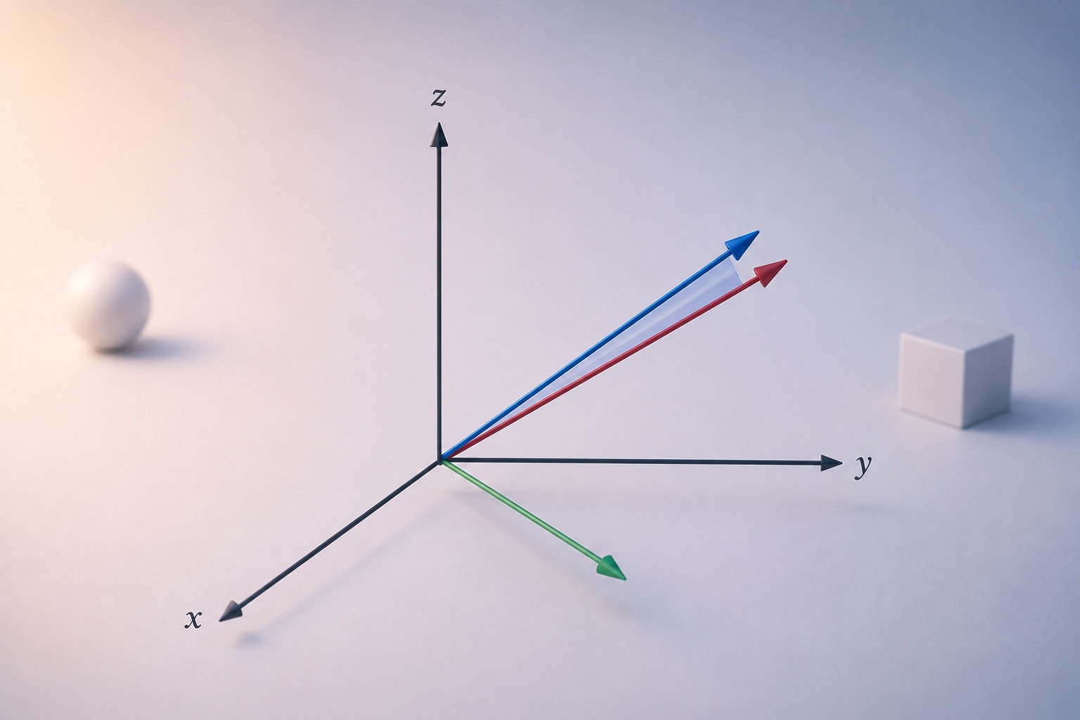
To know this, we have to cease pondering of options as columns of numbers and begin pondering of them as vectors in house. As soon as we do, multicollinearity stops being a statistical accident. It reveals itself as one thing else fully: a geometrical collapse, hiding in plain sight inside each regression you’ve ever run.

Part 3: The Hidden Geometry — Why Quantity Is Every little thing

We’ve seen the maths, and we’ve seen the mannequin’s identification disaster with Linear and Digital TV. However, as mentioned earlier than, to actually grasp why this occurs, we have to cease taking a look at rows of information and begin taking a look at vectors in house.

Multicollinearity isn’t a statistical glitch. It’s a bodily collapse of the house our mannequin lives in. And that’s what we’ll attempt to uncover now.

Earlier than we visualize this collapse, let’s shortly align on just a few basic instruments from linear algebra. They act because the mechanics of our regression, and we’d like them to observe the remainder of the story.
To observe the geometry of a failing mannequin, we have to maintain 4 ideas in thoughts:

The Transpose

Consider this as “flipping” our knowledge matrix. It’s a reorientation that permits us to carry out the following, most important step:

$X^T$

The Gram Matrix

After we multiply the transpose of X by itself, we aren’t simply doing algebra. We’re measuring inside merchandise. In plain English, it is a map of correlations. It tells us how a lot every characteristic factors in the identical course as each different:

$X^TX$

For our two TV channels, the off-diagonal entries of this matrix are basically a scaled correlation: how aligned Linear TV and Digital TV are throughout the weeks of our dataset.

The Determinant

In linear algebra, the determinant of a matrix is greater than only a complicated calculation. It’s a scaling issue and particularly, after we take a look at our Gram matrix, the determinant represents the quantity of the parallelepiped fashioned by our characteristic vectors in n-dimensional house.

The Inverse Constraint

For a novel answer of $hat{β}$ to exist, our Gram matrix should be invertible. That is solely potential if the determinant is non-zero:

$det(X^TX) > 0$

The nearer this determinant will get to zero, the extra our answer loses its footing.

The That means in Our Mannequin

Within the context of OLS regression, the determinant tells us how a lot distinctive house our variables really occupy.

Excessive Determinant (Stability)
If our options are impartial thus pointing in fully completely different instructions of their high-dimensional house then the field they kind is extensive open, with most quantity. Every characteristic contributes clear, distinct data to the mannequin. The system has sufficient impartial dimensions to pin each coefficient right down to a single, significant worth.

Low Determinant (Instability)
As correlation between options grows, the vectors begin to align. The field begins to tilt and flatten. Its quantity shrinks. The mannequin technically nonetheless has a novel answer, but it surely’s an answer sitting on a skinny sliver of house. It’s fragile, delicate, and straightforward to topple.

Zero Determinant (Collapse)
When collinearity is ideal (bear in mind our hypothetical linear_TV_v1 and linear_TV_v2 duplicate) the vectors lie precisely on high of one another. The n-dimensional quantity collapses right into a decrease dimension. A 3D field turns into a 2D aircraft. A 2D aircraft turns into a 1D line. The mannequin has no distinctive course left to decide on, and the maths provides up.

The Useless Finish
Why does a collapsing quantity break the maths? Recall our answer for $hat{β}$ from Half 1:

$hat{β} = (X^TX)^{-1} X^Ty$

To compute the inverse of the Gram matrix, we now have to divide the adjoint matrix by the determinant:

$displaystyle (X^TX)^{-1} = displaystyle frac{adj(X^TX}{det(X^TX)}$

If the determinant is zero, we’re fairly actually dividing by zero and thus no answer exists. However even when the determinant is simply very small (the practical case of strongly correlated channels), this division produces huge, unstable numbers. Tiny perturbations within the knowledge get amplified into monumental swings in $hat{β}$ .

That is the exact cause your coefficients explode. The mannequin isn’t malfunctioning. It’s making an attempt to stability itself on a geometrically vanishing floor and small ripples within the knowledge ship it sliding from +2.4 to +0.9 and again, each time you refresh the dataset.

A Visible Proof of the Collapse

To make this concrete, think about three advertising and marketing channels. Let’s say Linear TV, Digital TV, and a genuinely impartial third channel like Out-of-Residence (billboards, transit). When all three contribute impartial data, their vectors level in numerous instructions, and collectively they span a full three-dimensional quantity. The mannequin can comfortably distinguish their contributions.

However now suppose Digital TV is actually a scaled copy of Linear TV and so, they all the time transfer collectively, week after week. Geometrically, the Digital TV vector lies on the identical line because the Linear TV vector. Add the impartial OOH vector, and as a substitute of a 3D quantity we’re left with a flat 2D aircraft: two of our three “instructions” are actually the identical course.

That is the precise second the determinant collapses. The matrix loses an efficient dimension. The mannequin loses its grip.

The plot beneath reveals each situations facet by facet. In State of affairs A, three impartial characteristic vectors span a full 3D dice. In State of affairs B, the third vector is a linear mixture of the primary two vectors, geometrically pressured onto the identical 2D grey aircraft because the others. The 3D quantity vanishes. That is what near-collinearity appears like within the characteristic house and what zero determinant stands for.

From Geometry to Statistics

We’ve now seen, geometrically, why all the things falls aside when characteristic vectors crowd collectively: the quantity of the house our mannequin lives in shrinks towards zero, and the inverse of an almost-singular matrix produces wild, unstable solutions.

However this geometric image, stunning as it’s, lives one stage of abstraction away from the diagnostics we really use in follow. Once you match a regression in Python, you don’t see a determinant. You see customary errors. You see VIF scores. You see situation numbers in a mannequin abstract.

Within the subsequent part, we’ll translate this geometric collapse into the language of statistics — and watch the identical story unfold within the numbers that each knowledge scientist reads day-after-day.

Part 4: From Determinant to Variance

We’ve seen the geometric collapse. We’ve watched the quantity of our characteristic house shrink towards zero as Linear TV and Digital TV align. However right here’s a query that ought to trouble us: in our opening scene, I mentioned the director watched coefficients swing from +2.4 to +0.9. That’s not what a “damaged” mannequin appears like. A damaged mannequin would crash, throw a numerical error, refuse to suit. Our mannequin suits completely. It returns clear numbers. It simply returns completely different clear numbers each time the info shifts barely.

What does that imply, mathematically? The place precisely does the instability dwell?

The reply is hiding in a method that just about nobody talks about, however each statistician quietly is aware of:

$Var(hat{β}) = σ^2(Χ^ΤΧ)^{-1}$

That is the variance-covariance matrix of our OLS estimator. It tells us, for any given dataset, how a lot our estimated coefficients would fluctuate if we drew barely completely different samples from the identical underlying world. Its diagonal entries are the squared customary errors of every particular person $hat{β}$ , precisely the SE column you see in any regression abstract.

Take a look at the construction of this method rigorously. The variance of $hat{β}$ is proportional to the inverse of the Gram matrix. The exact same inverse we simply spent a complete part exhibiting collapses when options develop into correlated.

So the chain is clear and uncompromising:

Linear TV and Digital TV are almost collinear in our knowledge.
The columns of X are almost parallel vectors in remark house.
The amount of the parallelepiped they span is tiny.
$det(X^TX)$ could be very near zero.
$(X^TX)^{-1}$ has entries that blow up which means division by a near-zero quantity.
The diagonal of $(X^TX)^{-1}$ which is precisely $Var(hat{β})$ as much as a relentless turns into monumental.
The usual errors of our coefficients explode.

That is what your mannequin abstract is making an attempt to let you know, each time you see a regression output the place the coefficient is +2.4 however the usual error is ±2.1. The purpose estimate hasn’t moved by itself. What’s occurring is that the boldness interval round that estimate is so extensive that it comfortably accommodates +2.4 at this time, +0.9 tomorrow and -0.3 subsequent week and all of them statistically according to the identical underlying knowledge.

Your mannequin didn’t change its thoughts. It by no means had a thoughts made up within the first place. It simply had a confidence band extensive sufficient to swallow no matter particular quantity the newest dataset occurred to come out.

That is the exact statistical translation of geometric collapse. The amount of the characteristic house and the variance of the estimator aren’t two separate phenomena. They’re the identical truth, advised in numerous languages. One makes use of parallelepipeds whereas the opposite makes use of customary errors. Each are saying: we don’t have sufficient impartial data to pin this down.

And when you see this, each diagnostic in your regression output stops being mysterious. The usual errors. The extensive confidence intervals. The excessive p-values on coefficients ought to matter. None of those are bugs. They’re the mannequin, truthfully reporting again to you that the info isn’t telling it what you wished it will.

Within the subsequent part, we’ll see how this similar story will get translated yet one more time into the 2 diagnostics that knowledge scientists really attain for in follow: VIF and situation quantity.

Part 5: Similar Story, Two Extra Languages

By now, you’ve watched the identical phenomenon described in two completely different languages.

In geometric language: the characteristic vectors collapse towards a typical line, and the quantity of the house they span shrinks towards zero.

In statistical language: the variance of the estimator explodes, and customary errors develop into so extensive that at this time’s coefficient of +2.4 and tomorrow’s coefficient of +0.9 are equally according to the info.

VIF: How A lot of This Characteristic Is Already Mentioned by the Others?
However there’s a third language. That is the one your mannequin abstract really speaks whenever you match a regression in Python. It speaks in VIF scores and situation numbers. Most knowledge science programs train you to look at these numbers, apply some rule of thumb (VIF above 10 is dangerous), and transfer on. What not often will get defined is that these two diagnostics aren’t new data in any respect. They’re the very same story — the quantity collapse, the variance explosion — translated yet one more time, right into a kind you’ll be able to learn off a single line of code.

The Variance Inflation Issue for a characteristic is outlined as:

$VIF_i = frac{1}{1-R^2_i}$

The place $R^2_i$ is the coefficient of willpower you’d get if you happen to took a characteristic i — say, Linear TV — and regressed it towards all the opposite options in your mannequin equivalent to Digital TV, OOH, digital search, social media, and so forth.

Take some seconds to learn that definition once more. It’s asking a remarkably trustworthy query: how a lot of this characteristic will be predicted from the others? If Linear TV will be reconstructed virtually completely from the remainder of the channels (as a result of, say, Digital TV all the time strikes with it), then $R^2_i$ is near 1, the denominator $1-R^2_i$ approaches zero, and VIF explodes towards infinity.

When the options are genuinely impartial, $R^2_i=0$ , the denominator is 1, and VIF equals 1 — its decrease certain, indicating no inflation in any respect.

The identify itself tells the remainder of the story. Variance Inflation Issue. It’s actually measuring how a lot the variance of $hat{β_i}$ will get multiplied due to the characteristic’s overlap with the others. A VIF of 10 means the usual error of that coefficient is roughly $sqrt[]{10} simeq 3.2$ instances wider than it will be if the characteristic was impartial. A VIF of 100 means the usual error is 10 instances wider. The entire unhappy chain we walked via within the earlier part will get diminished to a single ratio you’ll be able to compute per characteristic.

VIF, then, just isn’t a separate idea. It’s the per-feature shadow of the geometric collapse: how a lot every particular person variable suffers from the truth that the others already cowl its territory.

Situation Quantity: The International Well being of the Matrix

The place VIF speaks to every characteristic individually, the situation quantity speaks to the matrix as an entire.

It comes from the Singular Worth Decomposition (SVD) of X. Any matrix will be decomposed right into a set of singular values $σ_1 ge σ_2 .. ge σ_p ge 0$ , which measure how a lot “stretch” the matrix applies alongside every of its principal instructions. Geometrically, these singular values are the lengths of the axes of the n-dimensional ellipsoid that X would carve out of a unit sphere.

The situation quantity is outlined as:

$κ(X) = frac{σ_{max}}{σ_{min}}$

When the options are impartial, the ellipsoid is roughly spherical thus all of the singular values are related in measurement, and their ratio is near 1. The matrix is well-rounded, balanced and wholesome.

When the options develop into almost collinear, the ellipsoid flattens. One course stretches enormously whereas one other collapses towards nothing. $σ_{min}$ shrinks towards zero, and the situation quantity explodes.

Discover that this is similar geometric collapse we already described, simply measured alongside a special axis. We beforehand mentioned: the quantity of the parallelepiped goes to zero. Now we’re saying: the shortest axis of the ellipsoid goes to zero. These aren’t two completely different info. The amount of a parallelepiped is the product of all of the singular values; if one among them collapses, the product collapses.

A typical rule of thumb: a situation quantity above 30 suggests severe multicollinearity. Above 100 is extreme. However the extra helpful instinct for me is that this: the situation quantity tells you, in a single quantity, how a lot numerical instability is baked into your design matrix earlier than you even begin becoming.

One Story, Three Languages

Step again for a second, and take a look at what we’ve constructed.

We began with a single phenomenon: when two options transfer collectively, a regression’s particular person coefficients develop into unstable. We then watched this phenomenon get described, in flip, by three completely different mathematical communities:

Geometers
Statisticians
Numerical Analysts

VIF and situation quantity aren’t additional diagnostics. They’re the operational summaries of the geometric fact we already understood. When you see this, the regression output stops being a mysterious desk of numbers and turns into a clear report on the geometric well being of your knowledge.

The subsequent time you see a VIF of 47 subsequent to a coefficient, you’ll know precisely what it means: that characteristic shares roughly an enormous portion of its variation with the others. The amount of impartial data it brings to the mannequin is sort of zero. The coefficient you see is the mannequin’s greatest guess from a vanishingly skinny slice of house.

Part 6: Watch It Occur – Code Demo

Let’s cease describing and begin watching. The cleanest solution to really feel multicollinearity is to assemble a tiny artificial case the place we management the correlation immediately, match an OLS regression, and skim the usual errors off the mannequin abstract.

The code beneath simulates a marketing-style dataset with three channels: Linear TV and Digital TV (which we’ll intentionally make correlated to various levels), and OOH as a genuinely impartial third channel. We then sweep the correlation between the 2 TV channels from delicate to near-perfect, match the identical regression every time, and watch what occurs.

import numpy as np 
import pandas as pd 
import statsmodels.api as sm 
np.random.seed(42) 
n_weeks = 200 

# True coefficients we're making an attempt to get better 
true_linear_tv = 2.0
true_digital_tv = 3.0 
true_ooh = 1.5 

outcomes = [] 
for corr in [0.3, 0.7, 0.9, 0.95, 0.99]: 
    # Linear TV: random weekly spend 
    linear_tv = np.random.uniform(0, 100, n_weeks) 

    # Digital TV: correlated with Linear TV, managed by `corr` 
    noise = np.random.regular(0, 1, n_weeks) 
    digital_tv = corr * linear_tv + np.sqrt(1 - corr**2) * noise * linear_tv.std() 
    # OOH: impartial 
    ooh = np.random.uniform(0, 50, n_weeks) 

    # Gross sales: true linear mixture + noise 
    gross sales = (true_linear_tv * linear_tv + 
                   true_digital_tv * digital_tv + 
                   true_ooh * ooh + 
                   np.random.regular(0, 30, n_weeks)) 

    X = sm.add_constant(np.column_stack([linear_tv, digital_tv, ooh])) 
    mannequin = sm.OLS(gross sales, X).match() 

    outcomes.append({ 'correlation': corr, 'beta_linear_tv': spherical(mannequin.params[1], 2),
           'SE_linear_tv': spherical(mannequin.bse[1], 2),
           'beta_digital_tv': spherical(mannequin.params[2], 2), 
           'SE_digital_tv': spherical(mannequin.bse[2], 2), 
           'beta_ooh': spherical(mannequin.params[3], 2), 
           'SE_ooh': spherical(mannequin.bse[3], 2), 
    })
print(pd.DataFrame(outcomes))

Because the correlation between Linear TV and Digital TV climbs from 0.3 to 0.99, the usual errors of each TV coefficients inflate dramatically from 0.08 to 0.56, roughly a sevenfold enhance. That is the variance explosion we derived analytically.

The purpose estimates themselves are fascinating to look at, too. At low correlation (0.3), the mannequin recovers the true values virtually completely: $hat{β}_{linearTV}=1.99$ towards a fact of two.0, and $hat{β}_{digitalTV}=3.01$ towards the reality of three.0. However by correlation 0.99, the estimates begin to drift visibly as Linear TV slides to 1.52 whereas Digital TV climbs to three.54. The purpose estimates haven’t gone insane, however they’ve began to slosh: the 2 coefficients are absorbing one another’s “credit score” as a result of the mannequin can now not cleanly attribute gross sales to at least one channel versus the opposite. The entire contribution stays roughly devoted; the person break up doesn’t.

And right here is the half that the usual errors quietly verify: at correlation 0.99, an ordinary error of 0.56 means the 95% confidence interval for Linear TV’s coefficient roughly spans from 0.4 to 2.6 which is extensive sufficient to include each the true worth and the drifted estimate, and virtually something in between. The mannequin just isn’t mendacity. It’s telling you, in its trustworthy statistical voice, that with this knowledge it can’t pin down particular person contributions with confidence.

Crucially, take a look at the OOH column. Throughout all the sweep — from correlation 0.3 to 0.99 — its coefficient stays anchored close to its true worth of 1.5, and its customary error barely budges. The illness is native to the correlated pair. That is precisely what the geometry predicted: the quantity of the characteristic house collapses solely within the instructions the place options pile on high of one another; in every single place else, the mannequin breathes freely.

Attempt enhancing one quantity on the high, both the random seed, the noise stage, the pattern measurement and rerun the code. The story is similar each time. As correlation rises, the usual errors of the correlated coefficients explode, and confidence in any particular person contribution dissolves. That is multicollinearity, now not described however noticed.

Part 7: The Final Lesson

Multicollinearity isn’t a query of damaged math. Your mannequin suits, your code runs, your output appears clear. The illness hides in the usual errors and in the best way coefficients quietly slosh from one quantity to a different between knowledge refreshes.

What we’ve seen is that this isn’t a statistical accident. It’s a geometric fact, dressed up in three completely different languages. When two options carry almost the identical data, the quantity of the house your mannequin lives in shrinks towards zero. The variance of the estimator inflates. VIF and situation quantity explode. These aren’t three separate issues. They’re one phenomenon, reported by three completely different communities of mathematicians who by no means fairly realized they have been all wanting on the similar factor.

The sensible responses are acquainted. Drop a characteristic, mix options, regularize. Every deserves its personal story. However none of them actually solves multicollinearity. They handle it. They acknowledge that the info has not given us sufficient impartial data, they usually discover principled methods to fill the hole.

So the following time a senior stakeholder asks you why your Linear TV coefficient was +2.4 yesterday and +0.9 at this time, you’ll have a greater reply than “the mannequin is delicate.” The reality is extra trustworthy, and extra fascinating. The characteristic house has flattened beneath your mannequin, and the coefficient you reported was the mannequin’s greatest guess from a skinny sliver of room. The quantity didn’t change as a result of the world did. It modified as a result of there was by no means fairly sufficient room for it to face nonetheless.