

# Introduction
Pandas is among the hottest Python libraries for information evaluation. It provides you easy instruments for cleansing, reshaping, summarizing, and exploring structured information. One of the crucial helpful options in pandas is GroupBy. It helps you reply questions that require grouping rows by a number of classes.
For instance, in case you are working with gross sales information, you could wish to calculate whole income by area, common order worth by product class, or the variety of orders dealt with by every gross sales consultant. As an alternative of manually filtering every class one after the other, GroupBy enables you to carry out these calculations in a clear and environment friendly approach.
On this tutorial, we’ll stroll via sensible examples of utilizing Pandas GroupBy with a small gross sales dataset. I’m utilizing Deepnote because the coding setting, so some outputs are proven as pocket book screenshots immediately beneath the code blocks.
# Making a Pattern Dataset
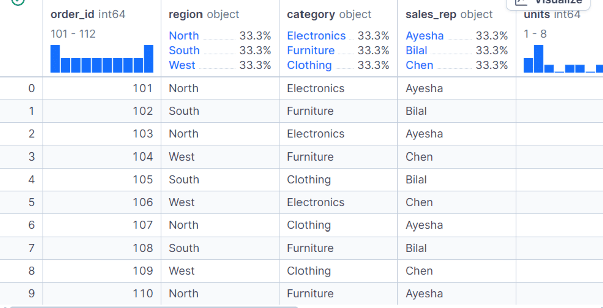
Earlier than utilizing GroupBy, we first create a small retail gross sales dataset with columns akin to order_id, area, class, sales_rep, models, unit_price, low cost, and order_date. We then convert the dictionary right into a pandas DataFrame and create two new columns: gross_sales and net_sales.
information = {
    "order_id": [101, 102, 103, 104, 105, 106, 107, 108, 109, 110, 111, 112],
    "area": ["North", "South", "North", "West", "South", "West", "North", "South", "West", "North", "South", "West"],
    "class": ["Electronics", "Furniture", "Electronics", "Furniture", "Clothing", "Electronics",
                 "Clothing", "Furniture", "Clothing", "Furniture", "Electronics", "Clothing"],
    "sales_rep": ["Ayesha", "Bilal", "Ayesha", "Chen", "Bilal", "Chen",
                  "Ayesha", "Bilal", "Chen", "Ayesha", "Bilal", "Chen"],
    "models": [2, 1, 3, 2, 5, 4, 6, 2, 7, 1, 2, 8],
    "unit_price": [500, 800, 450, 700, 60, 550, 55, 850, 65, 750, 520, 70],
    "low cost": [0.05, 0.10, 0.00, 0.08, 0.00, 0.12, 0.05, 0.10, 0.00, 0.07, 0.03, 0.00],
    "order_date": pd.to_datetime([
        "2026-01-05", "2026-01-06", "2026-01-08", "2026-01-10",
        "2026-01-12", "2026-01-15", "2026-02-02", "2026-02-05",
        "2026-02-08", "2026-02-12", "2026-02-15", "2026-02-20"
    ])
}

df = pd.DataFrame(information)

df["gross_sales"] = df["units"] * df["unit_price"]
df["net_sales"] = df["gross_sales"] * (1 - df["discount"])

df
The gross_sales column is calculated by multiplying models by unit_price, whereas net_sales adjusts that worth after making use of the low cost. This provides us a clear dataset that we will use for all GroupBy examples.
# Utilizing the Fundamental GroupBy Syntax
Essentially the most primary GroupBy operation follows a easy sample: choose a grouping column, choose the worth column, and apply an aggregation perform. On this instance, we group the information by area and calculate the full net_sales for every area.
df.groupby("area")["net_sales"].sum()
The end result exhibits that North, South, and West every have their very own whole gross sales worth. That is the best and most typical use case for GroupBy when summarizing information.
area
North    3311.0
South    3558.8
West     4239.0
Title: net_sales, dtype: float64
# Utilizing GroupBy With as_index=False
By default, pandas makes use of the grouped column because the index within the output. Whereas that is helpful in some circumstances, it’s typically simpler to work with a traditional DataFrame the place the grouped column stays an everyday column. That’s the place as_index=False is helpful.
df.groupby("area", as_index=False)["net_sales"].sum()
On this instance, we once more calculate whole internet gross sales by area, however the result’s returned as a clear DataFrame, which is less complicated to export, merge, or use in reviews.

# Making use of A number of Aggregations on One Column
GroupBy isn’t restricted to a single calculation. You’ll be able to apply a number of aggregation features to the identical column utilizing agg().
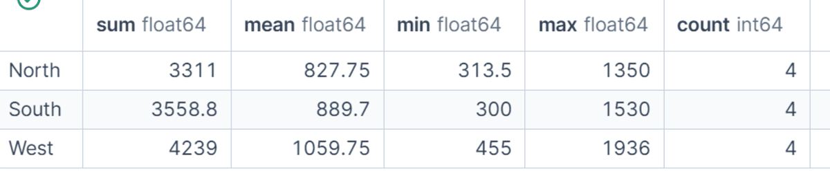
On this instance, we calculate the sum, imply, minimal, most, and depend of net_sales for every area.
This provides us a fast statistical abstract of regional gross sales efficiency and helps us examine not solely whole income but additionally common order dimension and order quantity.
df.groupby("area")["net_sales"].agg(["sum", "mean", "min", "max", "count"])
# Utilizing Named Aggregations
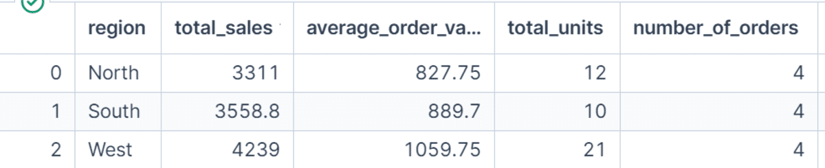
Named aggregations make GroupBy outputs simpler to learn and use. As an alternative of returning generic column names like sum or imply, we outline our personal names akin to total_sales, average_order_value, total_units, and number_of_orders.
That is particularly useful when getting ready evaluation for dashboards, reviews, or tutorials as a result of the output column names clearly clarify what every metric represents.
region_summary = (
    df.groupby("area", as_index=False)
      .agg(
          total_sales=("net_sales", "sum"),
          average_order_value=("net_sales", "imply"),
          total_units=("models", "sum"),
          number_of_orders=("order_id", "depend")
      )
)

region_summary
# Grouping by A number of Columns
You can even group information by a couple of column. On this instance, we group by each area and class to calculate whole internet gross sales for every product class inside every area.
This provides us a extra detailed view of the information in comparison with grouping by area alone. Multi-column grouping is helpful if you wish to analyze efficiency throughout completely different dimensions, akin to area and product, division and worker, or month and buyer section.
df.groupby(["region", "category"], as_index=False)["net_sales"].sum() 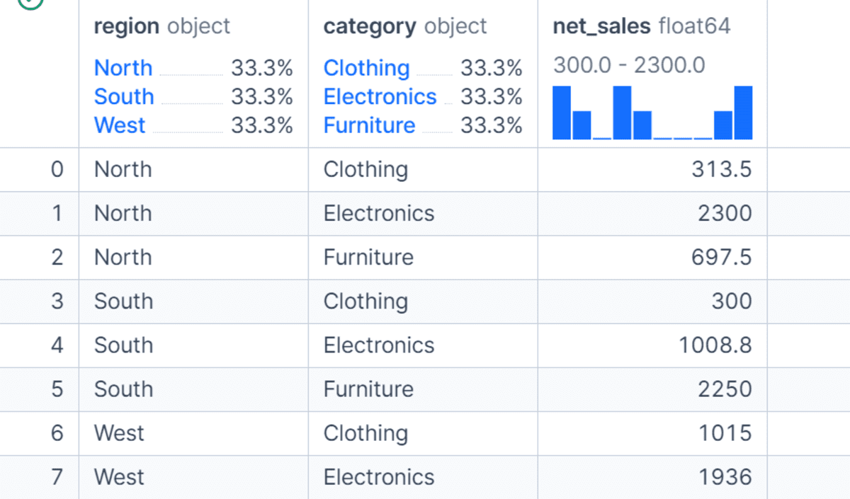
# Sorting GroupBy Outcomes
After grouping and aggregating information, you typically wish to kind the outcomes to seek out the very best or lowest values.
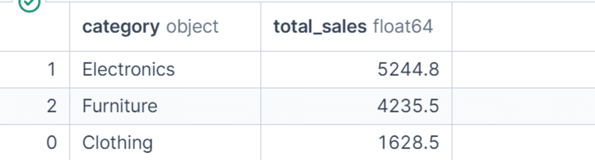
On this instance, we calculate whole gross sales by product class after which kind the leads to descending order.
This makes it straightforward to determine which class generated essentially the most income. Sorting grouped outcomes is an easy however highly effective step when turning uncooked summaries into helpful insights.
category_sales = (
    df.groupby("class", as_index=False)
      .agg(total_sales=("net_sales", "sum"))
      .sort_values("total_sales", ascending=False)
)

category_sales
# Understanding Depend vs Measurement
Pandas offers each depend() and dimension(), however they aren’t precisely the identical. The dimension() technique counts the full variety of rows in every group, together with rows with lacking values. The depend() technique counts solely non-missing values in a particular column.
On this instance, we deliberately add a lacking worth to the sales_rep column. The output exhibits that dimension() nonetheless counts 4 rows for every area, whereas depend() returns three for North as a result of one sales_rep worth is lacking.
import numpy as np

df_missing = df.copy()
df_missing.loc[2, "sales_rep"] = np.nan

print("Utilizing dimension():")
show(df_missing.groupby("area").dimension())

print("Utilizing depend() on sales_rep:")
show(df_missing.groupby("area")["sales_rep"].depend())
Output:
Utilizing dimension():
area
North    4
South    4
West     4
dtype: int64

Utilizing depend() on sales_rep:
area
North    3
South    4
West     4
Title: sales_rep, dtype: int64
# Utilizing remodel() for Group-Degree Options
The remodel() technique is helpful if you wish to calculate a group-level worth and add it again to the unique DataFrame.
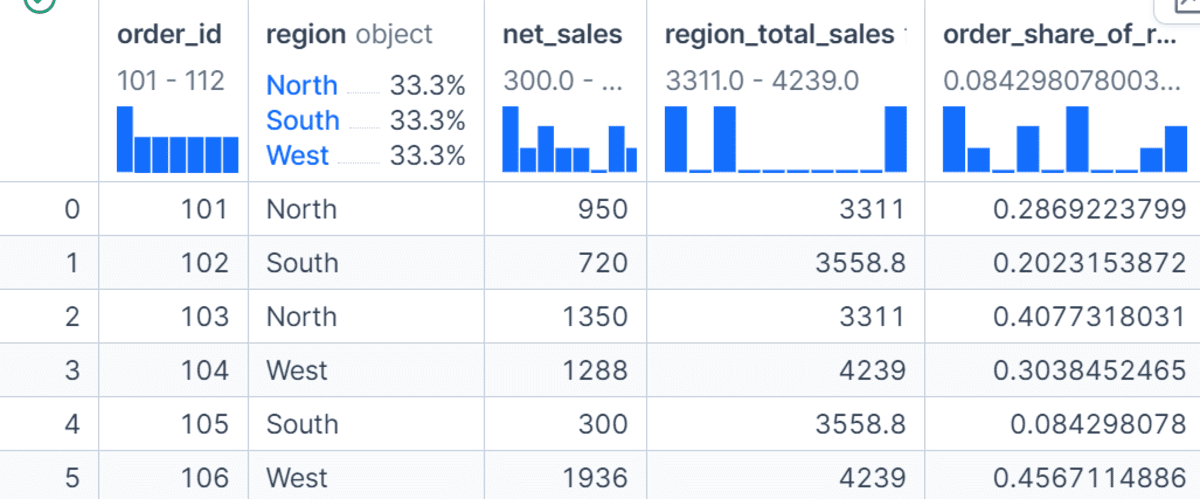
On this instance, we calculate whole gross sales for every area and retailer it in a brand new column referred to as region_total_sales.
We then calculate every order’s share of its area’s whole gross sales. Not like agg(), which reduces the information to 1 row per group, remodel() returns values aligned with the unique rows, making it very helpful for characteristic engineering.
df["region_total_sales"] = df.groupby("area")["net_sales"].remodel("sum")
df["order_share_of_region"] = df["net_sales"] / df["region_total_sales"]

df[["order_id", "region", "net_sales", "region_total_sales", "order_share_of_region"]]
# Filtering Teams With filter()
The filter() technique enables you to maintain or take away total teams based mostly on a situation. On this instance, we maintain solely the areas the place whole internet gross sales are better than 3,000.
As an alternative of returning one abstract row per group, filter() returns the unique rows from the teams that meet the situation. That is helpful if you wish to take away low-performing teams or maintain solely teams that fulfill a enterprise rule.
high_sales_regions = df.groupby("area").filter(lambda group: group["net_sales"].sum() > 3000)

high_sales_regions 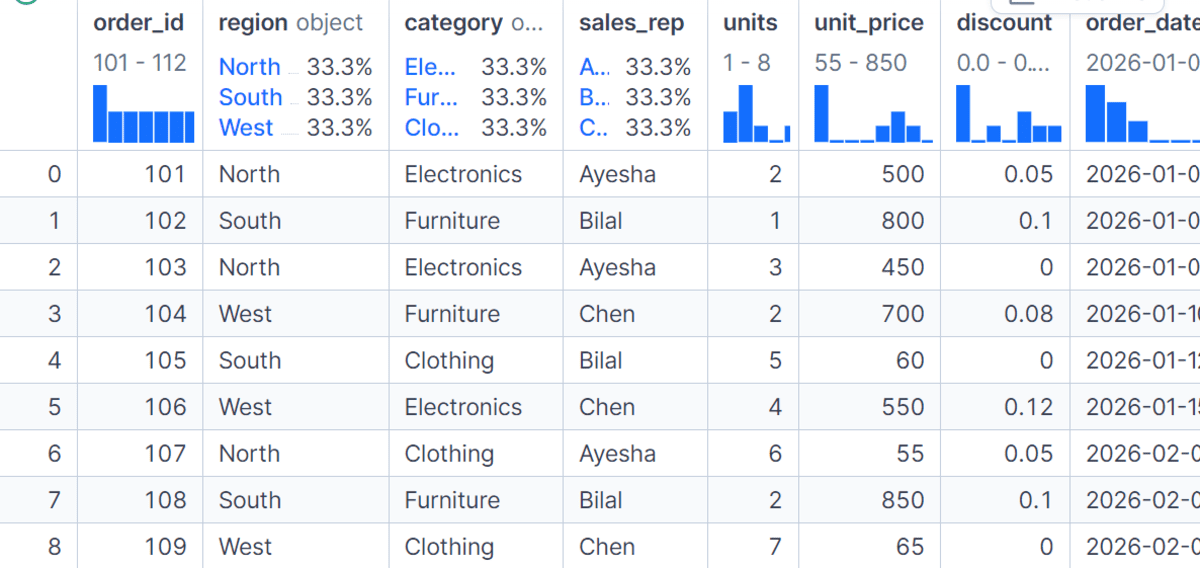
# Making use of Customized Logic With apply()
The apply() technique provides you extra flexibility as a result of it permits you to run customized logic on every group.
On this instance, we use apply() with nlargest() to seek out the highest order by internet gross sales in every area. That is helpful when built-in aggregation features usually are not sufficient on your evaluation.
Nevertheless, apply() might be slower than built-in strategies like sum(), imply(), agg(), and remodel(), so it’s best to make use of it solely if you want customized group-wise operations.
top_order_by_region = (
    df.groupby("area", group_keys=False)
      .apply(lambda group: group.nlargest(1, "net_sales"))
)

top_order_by_region

# Grouping by Dates
GroupBy can be very helpful for time-based evaluation.
On this instance, we extract the month from the order_date column and group the information by month.
We then calculate whole gross sales and whole orders for every month. This strategy is useful when analyzing traits over time, akin to month-to-month gross sales, weekly consumer exercise, or yearly income development.
df["month"] = df["order_date"].dt.to_period("M").astype(str)

monthly_sales = (
    df.groupby("month", as_index=False)
      .agg(total_sales=("net_sales", "sum"), total_orders=("order_id", "depend"))
)

monthly_sales

# Grouping by Dates With pd.Grouper
pd.Grouper offers a cleaner technique to group time sequence information with out manually making a separate month column.
On this instance, we group the DataFrame by order_date utilizing a month-to-month frequency and calculate whole gross sales and whole orders.
That is particularly helpful when working with real-world datasets that comprise timestamps and also you wish to summarize information by day, week, month, quarter, or yr.
monthly_sales_grouper = (
    df.groupby(pd.Grouper(key="order_date", freq="M"))
      .agg(total_sales=("net_sales", "sum"), total_orders=("order_id", "depend"))
      .reset_index()
)

monthly_sales_grouper 
# Making a Pivot-Fashion Abstract With GroupBy
You’ll be able to mix groupby() with unstack() to create a pivot-style abstract desk.
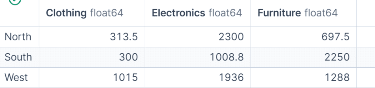
On this instance, we group the information by area and class, calculate whole internet gross sales, after which reshape the end result in order that classes develop into columns. This makes the output simpler to match throughout areas and classes. It’s a nice method if you need a compact desk for reporting or fast evaluation.
region_category_table = (
    df.groupby(["region", "category"])["net_sales"]
      .sum()
      .unstack(fill_value=0)
)

region_category_table
# Conclusion
Pandas GroupBy is among the strongest instruments for information evaluation in Python. It helps you summarize information, examine teams, create new options, filter outcomes, and apply customized calculations with out writing pointless guide logic.
Whereas engaged on this tutorial, I spotted how a lot depth there may be in GroupBy. Even after working with information for years, I discovered new and higher methods to resolve widespread issues. Options like pd.Grouper, customized aggregation features, and remodel() stood out as a result of they make many duties sooner, cleaner, and simpler to take care of.
That is additionally why understanding the native instruments issues. It’s tempting to depend on vibe coding or fast customized options, however these can typically produce slower, extra sophisticated code. When what pandas already offers, you possibly can write options which might be extra environment friendly, reusable, and sensible for real-world information evaluation.
On this tutorial, we coated essentially the most helpful GroupBy operations, together with primary aggregation, named aggregation, multi-column grouping, sorting, depend() vs dimension(), remodel(), filter(), apply(), date grouping, and pivot-style summaries. When you perceive these patterns, you should use GroupBy to reply many real-world information evaluation questions rapidly and confidently.
Abid Ali Awan (@1abidaliawan) is a licensed information scientist skilled who loves constructing machine studying fashions. At present, he’s specializing in content material creation and writing technical blogs on machine studying and information science applied sciences. Abid holds a Grasp’s diploma in expertise administration and a bachelor’s diploma in telecommunication engineering. His imaginative and prescient is to construct an AI product utilizing a graph neural community for college students battling psychological sickness.
# Introduction
Pandas is among the hottest Python libraries for information evaluation. It provides you easy instruments for cleansing, reshaping, summarizing, and exploring structured information. One of the crucial helpful options in pandas is GroupBy. It helps you reply questions that require grouping rows by a number of classes.
For instance, in case you are working with gross sales information, you could wish to calculate whole income by area, common order worth by product class, or the variety of orders dealt with by every gross sales consultant. As an alternative of manually filtering every class one after the other, GroupBy enables you to carry out these calculations in a clear and environment friendly approach.
On this tutorial, we’ll stroll via sensible examples of utilizing Pandas GroupBy with a small gross sales dataset. I’m utilizing Deepnote because the coding setting, so some outputs are proven as pocket book screenshots immediately beneath the code blocks.
# Making a Pattern Dataset
Earlier than utilizing GroupBy, we first create a small retail gross sales dataset with columns akin to order_id, area, class, sales_rep, models, unit_price, low cost, and order_date. We then convert the dictionary right into a pandas DataFrame and create two new columns: gross_sales and net_sales.
information = {
    "order_id": [101, 102, 103, 104, 105, 106, 107, 108, 109, 110, 111, 112],
    "area": ["North", "South", "North", "West", "South", "West", "North", "South", "West", "North", "South", "West"],
    "class": ["Electronics", "Furniture", "Electronics", "Furniture", "Clothing", "Electronics",
                 "Clothing", "Furniture", "Clothing", "Furniture", "Electronics", "Clothing"],
    "sales_rep": ["Ayesha", "Bilal", "Ayesha", "Chen", "Bilal", "Chen",
                  "Ayesha", "Bilal", "Chen", "Ayesha", "Bilal", "Chen"],
    "models": [2, 1, 3, 2, 5, 4, 6, 2, 7, 1, 2, 8],
    "unit_price": [500, 800, 450, 700, 60, 550, 55, 850, 65, 750, 520, 70],
    "low cost": [0.05, 0.10, 0.00, 0.08, 0.00, 0.12, 0.05, 0.10, 0.00, 0.07, 0.03, 0.00],
    "order_date": pd.to_datetime([
        "2026-01-05", "2026-01-06", "2026-01-08", "2026-01-10",
        "2026-01-12", "2026-01-15", "2026-02-02", "2026-02-05",
        "2026-02-08", "2026-02-12", "2026-02-15", "2026-02-20"
    ])
}

df = pd.DataFrame(information)

df["gross_sales"] = df["units"] * df["unit_price"]
df["net_sales"] = df["gross_sales"] * (1 - df["discount"])

df
The gross_sales column is calculated by multiplying models by unit_price, whereas net_sales adjusts that worth after making use of the low cost. This provides us a clear dataset that we will use for all GroupBy examples.
# Utilizing the Fundamental GroupBy Syntax
Essentially the most primary GroupBy operation follows a easy sample: choose a grouping column, choose the worth column, and apply an aggregation perform. On this instance, we group the information by area and calculate the full net_sales for every area.
df.groupby("area")["net_sales"].sum()
The end result exhibits that North, South, and West every have their very own whole gross sales worth. That is the best and most typical use case for GroupBy when summarizing information.
area
North    3311.0
South    3558.8
West     4239.0
Title: net_sales, dtype: float64
# Utilizing GroupBy With as_index=False
By default, pandas makes use of the grouped column because the index within the output. Whereas that is helpful in some circumstances, it’s typically simpler to work with a traditional DataFrame the place the grouped column stays an everyday column. That’s the place as_index=False is helpful.
df.groupby("area", as_index=False)["net_sales"].sum()
On this instance, we once more calculate whole internet gross sales by area, however the result’s returned as a clear DataFrame, which is less complicated to export, merge, or use in reviews.
# Making use of A number of Aggregations on One Column
GroupBy isn’t restricted to a single calculation. You’ll be able to apply a number of aggregation features to the identical column utilizing agg().
On this instance, we calculate the sum, imply, minimal, most, and depend of net_sales for every area.
This provides us a fast statistical abstract of regional gross sales efficiency and helps us examine not solely whole income but additionally common order dimension and order quantity.
df.groupby("area")["net_sales"].agg(["sum", "mean", "min", "max", "count"])
# Utilizing Named Aggregations
Named aggregations make GroupBy outputs simpler to learn and use. As an alternative of returning generic column names like sum or imply, we outline our personal names akin to total_sales, average_order_value, total_units, and number_of_orders.
That is particularly useful when getting ready evaluation for dashboards, reviews, or tutorials as a result of the output column names clearly clarify what every metric represents.
region_summary = (
    df.groupby("area", as_index=False)
      .agg(
          total_sales=("net_sales", "sum"),
          average_order_value=("net_sales", "imply"),
          total_units=("models", "sum"),
          number_of_orders=("order_id", "depend")
      )
)

region_summary
# Grouping by A number of Columns
You can even group information by a couple of column. On this instance, we group by each area and class to calculate whole internet gross sales for every product class inside every area.
This provides us a extra detailed view of the information in comparison with grouping by area alone. Multi-column grouping is helpful if you wish to analyze efficiency throughout completely different dimensions, akin to area and product, division and worker, or month and buyer section.
df.groupby(["region", "category"], as_index=False)["net_sales"].sum()
# Sorting GroupBy Outcomes
After grouping and aggregating information, you typically wish to kind the outcomes to seek out the very best or lowest values.
On this instance, we calculate whole gross sales by product class after which kind the leads to descending order.
This makes it straightforward to determine which class generated essentially the most income. Sorting grouped outcomes is an easy however highly effective step when turning uncooked summaries into helpful insights.
category_sales = (
    df.groupby("class", as_index=False)
      .agg(total_sales=("net_sales", "sum"))
      .sort_values("total_sales", ascending=False)
)

category_sales
# Understanding Depend vs Measurement
Pandas offers each depend() and dimension(), however they aren’t precisely the identical. The dimension() technique counts the full variety of rows in every group, together with rows with lacking values. The depend() technique counts solely non-missing values in a particular column.
On this instance, we deliberately add a lacking worth to the sales_rep column. The output exhibits that dimension() nonetheless counts 4 rows for every area, whereas depend() returns three for North as a result of one sales_rep worth is lacking.
import numpy as np

df_missing = df.copy()
df_missing.loc[2, "sales_rep"] = np.nan

print("Utilizing dimension():")
show(df_missing.groupby("area").dimension())

print("Utilizing depend() on sales_rep:")
show(df_missing.groupby("area")["sales_rep"].depend())
Output:
Utilizing dimension():
area
North    4
South    4
West     4
dtype: int64

Utilizing depend() on sales_rep:
area
North    3
South    4
West     4
Title: sales_rep, dtype: int64
# Utilizing remodel() for Group-Degree Options
The remodel() technique is helpful if you wish to calculate a group-level worth and add it again to the unique DataFrame.
On this instance, we calculate whole gross sales for every area and retailer it in a brand new column referred to as region_total_sales.
We then calculate every order’s share of its area’s whole gross sales. Not like agg(), which reduces the information to 1 row per group, remodel() returns values aligned with the unique rows, making it very helpful for characteristic engineering.
df["region_total_sales"] = df.groupby("area")["net_sales"].remodel("sum")
df["order_share_of_region"] = df["net_sales"] / df["region_total_sales"]

df[["order_id", "region", "net_sales", "region_total_sales", "order_share_of_region"]]
# Filtering Teams With filter()
The filter() technique enables you to maintain or take away total teams based mostly on a situation. On this instance, we maintain solely the areas the place whole internet gross sales are better than 3,000.
As an alternative of returning one abstract row per group, filter() returns the unique rows from the teams that meet the situation. That is helpful if you wish to take away low-performing teams or maintain solely teams that fulfill a enterprise rule.
high_sales_regions = df.groupby("area").filter(lambda group: group["net_sales"].sum() > 3000)

high_sales_regions
# Making use of Customized Logic With apply()
The apply() technique provides you extra flexibility as a result of it permits you to run customized logic on every group.
On this instance, we use apply() with nlargest() to seek out the highest order by internet gross sales in every area. That is helpful when built-in aggregation features usually are not sufficient on your evaluation.
Nevertheless, apply() might be slower than built-in strategies like sum(), imply(), agg(), and remodel(), so it’s best to make use of it solely if you want customized group-wise operations.
top_order_by_region = (
    df.groupby("area", group_keys=False)
      .apply(lambda group: group.nlargest(1, "net_sales"))
)

top_order_by_region
# Grouping by Dates
GroupBy can be very helpful for time-based evaluation.
On this instance, we extract the month from the order_date column and group the information by month.
We then calculate whole gross sales and whole orders for every month. This strategy is useful when analyzing traits over time, akin to month-to-month gross sales, weekly consumer exercise, or yearly income development.
df["month"] = df["order_date"].dt.to_period("M").astype(str)

monthly_sales = (
    df.groupby("month", as_index=False)
      .agg(total_sales=("net_sales", "sum"), total_orders=("order_id", "depend"))
)

monthly_sales
# Grouping by Dates With pd.Grouper
pd.Grouper offers a cleaner technique to group time sequence information with out manually making a separate month column.
On this instance, we group the DataFrame by order_date utilizing a month-to-month frequency and calculate whole gross sales and whole orders.
That is particularly helpful when working with real-world datasets that comprise timestamps and also you wish to summarize information by day, week, month, quarter, or yr.
monthly_sales_grouper = (
    df.groupby(pd.Grouper(key="order_date", freq="M"))
      .agg(total_sales=("net_sales", "sum"), total_orders=("order_id", "depend"))
      .reset_index()
)

monthly_sales_grouper
# Making a Pivot-Fashion Abstract With GroupBy
You’ll be able to mix groupby() with unstack() to create a pivot-style abstract desk.
On this instance, we group the information by area and class, calculate whole internet gross sales, after which reshape the end result in order that classes develop into columns. This makes the output simpler to match throughout areas and classes. It’s a nice method if you need a compact desk for reporting or fast evaluation.
region_category_table = (
    df.groupby(["region", "category"])["net_sales"]
      .sum()
      .unstack(fill_value=0)
)

region_category_table
# Conclusion
Pandas GroupBy is among the strongest instruments for information evaluation in Python. It helps you summarize information, examine teams, create new options, filter outcomes, and apply customized calculations with out writing pointless guide logic.
Whereas engaged on this tutorial, I spotted how a lot depth there may be in GroupBy. Even after working with information for years, I discovered new and higher methods to resolve widespread issues. Options like pd.Grouper, customized aggregation features, and remodel() stood out as a result of they make many duties sooner, cleaner, and simpler to take care of.
That is additionally why understanding the native instruments issues. It’s tempting to depend on vibe coding or fast customized options, however these can typically produce slower, extra sophisticated code. When what pandas already offers, you possibly can write options which might be extra environment friendly, reusable, and sensible for real-world information evaluation.
On this tutorial, we coated essentially the most helpful GroupBy operations, together with primary aggregation, named aggregation, multi-column grouping, sorting, depend() vs dimension(), remodel(), filter(), apply(), date grouping, and pivot-style summaries. When you perceive these patterns, you should use GroupBy to reply many real-world information evaluation questions rapidly and confidently.
Abid Ali Awan (@1abidaliawan) is a licensed information scientist skilled who loves constructing machine studying fashions. At present, he’s specializing in content material creation and writing technical blogs on machine studying and information science applied sciences. Abid holds a Grasp’s diploma in expertise administration and a bachelor’s diploma in telecommunication engineering. His imaginative and prescient is to construct an AI product utilizing a graph neural community for college students battling psychological sickness.