Hybrid Search and Re-Rating in Manufacturing RAG

Studying Phrase Vectors for Sentiment Evaluation: A Python Copy

Batch or Stream? The Everlasting Information Processing Dilemma

, we bought a grievance from certainly one of our platform engineers of the infrastructure staff that our inner information assistant is confidently giving the improper solutions when requested concerning the retry coverage for our message-queue customers. It seems to be like a easy query, and the assistant ought to have given a well-documented reply, however I used to be improper.

The system returned a three-paragraph response about exponential backoff with jitter. All of it was correct however none of it was what she requested for. The precise doc she wished described a customized override we had put in place for one particular service after a manufacturing incident that hit us six months earlier. The doc used the phrase “dead-letter queue threshold” repeatedly. Our embedding mannequin had determined that “exponential backoff” and “dead-letter queue threshold” have been semantically shut sufficient.

I checked the retrieval logs and came upon that the doc she wanted was sitting at place eleven within the outcomes simply exterior the highest ten that have been handed to the mannequin. The system had not didn’t index or retrieve it however it was ranked beneath ten different paperwork.

The Drawback With Dense Vectors

That is half 3 of The RAG for Enterprise collection, and when you have missed the sooner elements I might strongly advocate you to verify them out first: A sensible information to RAG for Enterprise Information base and Your Chunks Failed Your RAG in Manufacturing

Dense retrieval works by changing textual content into high-dimensional vectors and discovering the chunks whose vectors are geometrically near the question vector. If two items of textual content means contextually comparable issues, their vectors ought to find yourself close by in embedding area.

This holds nicely for conceptual queries equivalent to “What’s our incident escalation course of?”. This question will retrieve incident associated paperwork even when the doc makes use of the phrases like “severity triage” as an alternative of “escalation.” The embedding mannequin has discovered that these ideas are associated, and cosine similarity captures that.

The issue come up when the particular technical language comes into play. An engineer looking for “dead-letter queue threshold configuration” is just not asking a conceptual query. She needs the precise time period from the precise doc however the embedding illustration of “dead-letter queue threshold” has been averaged out by every part else within the surrounding paragraphs right into a single dense vector. This averaging is a commerce off. The identical property that makes dense retrieval good at conceptual matching makes it unreliable for precise time period lookup.

Bi-encoders, the fashions that energy dense retrieval, compress the that means of a complete chunk into one fixed-size vector. This compression loses data. The query is just not whether or not any data ought to be misplaced or not however which data we will afford to lose.

BM25: what’s at and the way does it assist

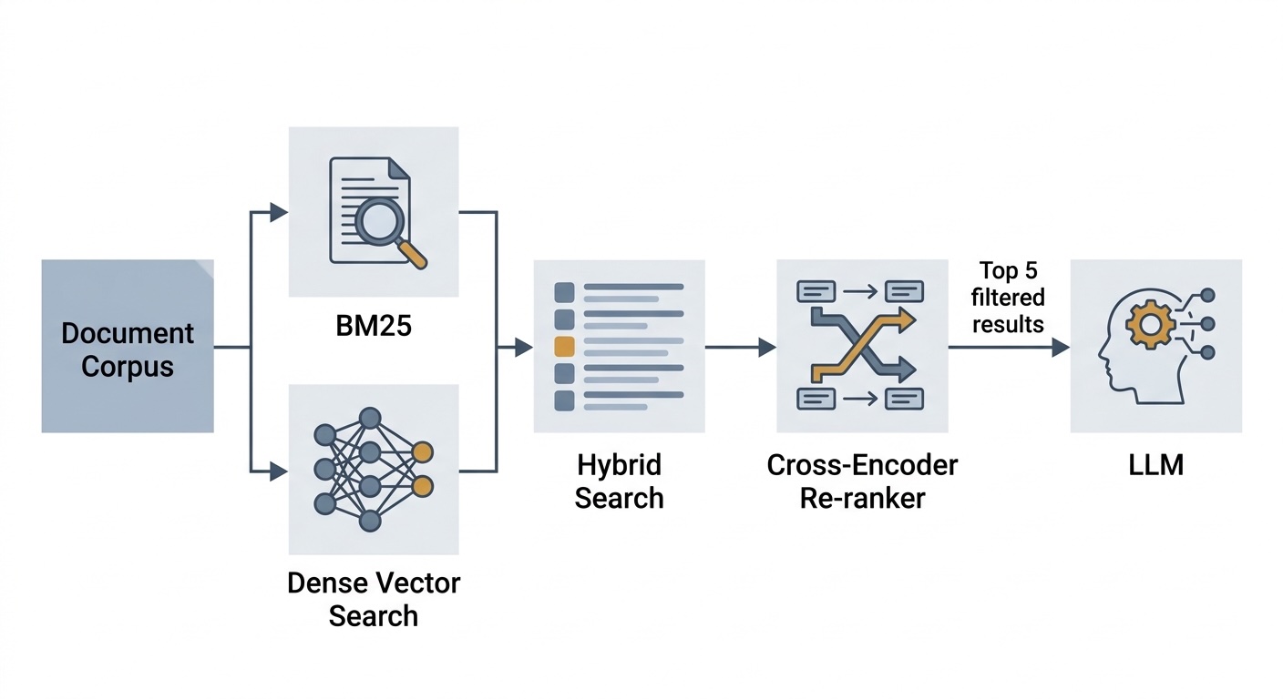
Earlier than neural retrieval existed, search was dominated by time period frequency strategies. BM25, or Greatest Match 25, is likely one of the greatest strategies on the market and it’s extensively utilized in Elasticsearch, Solr, Weaviate, and most manufacturing search techniques.

BM25 scores a doc in opposition to a question by taking a look at it from a number of instructions. Its foremost parts are:

The IDF part, which asks itself how tough it’s to discover a time period wherever within the corpus. A time period that seems in majority of the paperwork tells us nearly nothing about relevance. “Lifeless-letter queue threshold” showing in only some paperwork is a robust sign. IDF offers uncommon phrases extra weightage.

The time period frequency part asks how usually the time period seems on this particular doc. Right here BM25 will get intelligent and applies a saturation operate reasonably than simply utilizing the uncooked frequency. Due to this saturation operate the rating grows quickly within the beginning after which flattens.

The size normalisation part penalises longer paperwork. An extended doc naturally incorporates extra time period occurrences. With out normalisation it might floor the longest paperwork which isn’t what we wish.

BM25 can’t match synonyms, deal with paraphrases, or perceive that “configuration override” and “customized settings” are associated. It’s a bag-of-words mannequin and phrase order and semantics don’t matter to it. The phrase “the configuration overrides the default retry behaviour” and “the default retry behaviour could be overridden by way of configuration” are similar to BM25 and that’s each its power and its limitation.

Hybrid Search: Combining Each

Weaviate helps hybrid search natively, combining BM25 key phrase scores and dense vector similarity scores right into a single ranked listing by a way known as Relative Rating Fusion. The important thing parameter is alpha which controls the mix. An alpha of 1 is pure vector search and an alpha of 0 is pure BM25. All the pieces between is a weighted mixture.

from llama_index.core.retrievers import VectorIndexRetriever
from llama_index.core.vector_stores import MetadataFilter, MetadataFilters

# Alpha of 0.5 = equal weight to key phrase and semantic alerts
retriever = VectorIndexRetriever(
    index=index,
    similarity_top_k=10,
    vector_store_query_mode="hybrid",
    alpha=0.5,
    vector_store_kwargs={
        "filters": MetadataFilters(filters=[
            MetadataFilter(key="department", value="engineering")
        ])
    }
)

That is the straightforward half, however deciding what alpha worth to make use of is the tougher half.

The query is how exact your typical question is. If most of your queries are conceptual (“how does our incident course of work?”), larger alpha tilts you towards semantic matching. If queries are sometimes exact-term lookups (“GDPR Article 17 guidelines”, “retry coverage DLQ threshold”, “Service X SLA”), decrease alpha offers extra weight to key phrase matching.

In follow, you need to measure it as an alternative of simply guessing. Right here is how I tuned alpha on our corpus utilizing a labelled analysis set of 150 query-document pairs drawn from our IT helpdesk historical past.

import ragas
from ragas.metrics import ContextPrecision, ContextRecall
from datasets import Dataset
import numpy as np

def evaluate_alpha(alpha_value, eval_queries, ground_truth_docs):
    outcomes = []
    for question, expected_doc_ids in zip(eval_queries, ground_truth_docs):
        # Replace retriever with new alpha
        retriever.alpha = alpha_value
        retrieved_nodes = retriever.retrieve(question)
        retrieved_ids = [n.node.metadata.get("doc_id") for n in retrieved_nodes]

        hit = any(doc_id in retrieved_ids for doc_id in expected_doc_ids)
        rank = subsequent(
            (i + 1 for i, doc_id in enumerate(retrieved_ids) if doc_id in expected_doc_ids),
            None
        )
        outcomes.append({"hit": hit, "rank": rank})
    
    hit_rate = np.imply([r["hit"] for r in outcomes])
    mrr = np.imply([1 / r["rank"] if r["rank"] else 0 for r in outcomes])
    return {"alpha": alpha_value, "hit_rate": hit_rate, "mrr": mrr}

# Check throughout the vary
alphas = [0.0, 0.25, 0.5, 0.75, 1.0]
outcomes = [evaluate_alpha(a, eval_queries, ground_truth_docs) for a in alphas]

for r in outcomes:
    print(f"Alpha: {r['alpha']:.2f} | Hit Price: {r['hit_rate']:.3f} | MRR: {r['mrr']:.3f}")

On our engineering corpus, the outcomes appeared like this (your numbers will differ):

Alpha: 0.00 | Hit Price: 0.71 | MRR: 0.58    # Pure BM25
Alpha: 0.25 | Hit Price: 0.80 | MRR: 0.66
Alpha: 0.50 | Hit Price: 0.83 | MRR: 0.69    -> our candy spot
Alpha: 0.75 | Hit Price: 0.81 | MRR: 0.67
Alpha: 1.00 | Hit Price: 0.73 | MRR: 0.61    # Pure dense

The pure modes have been clearly worse than any mix. The dead-letter queue question that had failed earlier than moved from rank eleven to rank 4 at 0.5 alpha, as a result of the BM25 sign pulled it up despite the fact that the dense sign was nonetheless ambivalent.

An vital caveat on these numbers: in case your corpus is generally long-form narrative documentation, you may discover that 0.65 – 0.75 alpha works higher. If it incorporates lots of precise technical identifiers, error codes, product names, 0.35 – 0.5 will doubtless serve you higher. There isn’t any common appropriate worth. Measure by yourself knowledge.

Observe: In case your Hit Price at alpha=0.0 (pure BM25) is considerably decrease than at alpha=1.0 (pure dense), your corpus has vocabulary-rich content material with paraphrase, on this case you must lean in direction of larger alpha. If the reverse is true, your customers search with exact technical phrases then you must lean in direction of decrease alpha. If they’re comparable, begin at 0.5 and tune it from there.

The Drawback that Hybrid Search Does Not Resolve

Once you move ten retrieved chunks to an LLM, it reads all of them. However its consideration is just not uniform throughout the context window. A number of research just like the “misplaced within the center” downside have proven that fashions pay extra consideration to context close to the start and finish of their enter and are much less dependable about data buried within the center. If essentially the most related chunk is sitting at place eight of ten, you’re counting on the mannequin to fish it out from a comparatively inattentive zone.

Cross-Encoders: What They Are and Why They Work

A bi-encoder processes the question and the doc utterly independently. By the point it computes similarity, the 2 finalised vectors doesn’t is aware of concerning the different.

A cross-encoder does one thing completely different. It takes the question and a single doc, concatenates them into one enter sequence, and runs them by the transformer collectively. Each consideration layer within the mannequin can now let question tokens attend to doc tokens and vice versa. The mannequin sees the total interplay between the 2 earlier than producing its relevance rating.

The distinction in what the mannequin can detect is substantial. Take into account the question “What’s the retry restrict for the cost service?” and two candidate chunks: “Retry limits fluctuate by service sort. For many inner providers, the default is three makes an attempt with exponential backoff.” and “The cost service client is configured with a most of 5 retry makes an attempt earlier than the message is routed to the dead-letter queue.”

A bi-encoder may rank Chunk A better as a result of “retry restrict” and “retry limits fluctuate by service sort” are semantically shut. A cross-encoder studying each texts collectively instantly notices that Chunk B incorporates the precise quantity for the particular service the question asks about. The cross-attention between “cost service” within the question and “cost service client” within the doc offers it direct proof that Chunk B is the correct reply.

For this reason cross-encoders are considerably extra correct than bi-encoders on rating duties. The limitation is that they can not pre-compute something. A bi-encoder can pre-embed all of your paperwork at index time after which simply embed the question at search time therefore performing two operations. A cross-encoder should course of each (question, doc) pair at question time. For 1,000,000 paperwork, that could be a million ahead passes. You can not run a cross-encoder over your whole corpus.

The answer is the two-stage funnel: use the bi-encoder to forged a large web and retrieve the highest N candidates rapidly, then use the cross-encoder to re-score solely these N candidates exactly.

In follow, the cross-encoder provides roughly 80 – 120 ms to question latency when re-ranking 20 paperwork with a light-weight mannequin on CPU.

Implementing Re-ranking

We use ms-marco-MiniLM-L-6-v2 from the sentence-transformers library. It was skilled on MS MARCO, a large-scale query answering dataset, and it’s the most generally used open-source cross-encoder for common retrieval duties. For domain-specific content material you’ll be able to fine-tune by yourself labelled pairs, however the common mannequin is an inexpensive place to begin.

from sentence_transformers import CrossEncoder

reranker = CrossEncoder("cross-encoder/ms-marco-MiniLM-L-6-v2")

def rerank_nodes(question: str, retrieved_nodes: listing, top_n: int = 5) -> listing:
    """
    Takes question and a listing of LlamaIndex NodeWithScore objects,
    returns top_n nodes reranked by cross-encoder rating.
    """
    # Construct (question, chunk_text) pairs for the cross-encoder
    pairs = [(query, node.node.get_content()) for node in retrieved_nodes]
    
    # Rating all pairs and returns a listing of floats
    scores = reranker.predict(pairs)
    
    # Connect scores to nodes and kind
    for node, rating in zip(retrieved_nodes, scores):
        node.rating = float(rating)
    
    reranked = sorted(retrieved_nodes, key=lambda n: n.rating, reverse=True)
    return reranked[:top_n]


# Full retrieval + re-ranking pipeline
question = "What's the retry restrict for the cost service dead-letter queue?"

# Stage 1: retrieve greater than you want (20 candidates)
retrieved = retriever.retrieve(question)   # top_k=20 in retriever config

# Stage 2: re-rank down to five
reranked = rerank_nodes(question, retrieved, top_n=5)

# Examine what occurred to doc ranks
print("After re-ranking:")
for i, node in enumerate(reranked):
    supply = node.node.metadata.get("supply", "unknown")
    print(f"  Rank {i+1} | Rating: {node.rating:.4f} | Supply: {supply}")

LlamaIndex additionally has a local SentenceTransformerRerank post-processor that integrates into its question pipeline cleanly:

from llama_index.postprocessor.sbert_rerank import SentenceTransformerRerank
from llama_index.core import QueryBundle
from llama_index.core.query_engine import RetrieverQueryEngine

reranker_postprocessor = SentenceTransformerRerank(
    mannequin="cross-encoder/ms-marco-MiniLM-L-6-v2",
    top_n=5
)

query_engine = RetrieverQueryEngine.from_args(
    retriever=retriever,
    node_postprocessors=[reranker_postprocessor]
)

response = query_engine.question(
    "What's the retry restrict for the cost service dead-letter queue?"
)

top_n=5 right here tells the reranker what number of paperwork to move to the era step. Growing this provides the LLM extra context however will increase each latency and the danger of noise. In our system, 5 was the candy spot, sufficient context for multi-part questions with out cluttering the immediate.

Observe: Log the rank correlation between retrieval order and re-ranking order throughout a pattern of queries. If the cross-encoder isn’t altering the rating, both your bi-encoder is already doing a great job and re-ranking provides little worth, or your cross-encoder mannequin is simply too generic on your area.

Measuring the Influence

We’re evaluating the three issues collectively, pure dense retrieval (our baseline), hybrid search, and hybrid + re-ranking. I ran our analysis set of 150 queries by all three configurations.

from ragas import consider
from ragas.metrics import (
    ContextPrecision,
    ContextRecall,
    AnswerRelevancy,
    Faithfulness
)
from datasets import Dataset

def build_ragas_dataset(queries, retrieved_contexts, ground_truths, generated_answers):
    return Dataset.from_dict({
        "query": queries,
        "contexts": retrieved_contexts,    # listing of lists of strings
        "reply": generated_answers,
        "ground_truth": ground_truths
    })

# Construct datasets for every configuration, then consider
baseline_dataset = build_ragas_dataset(
    queries, baseline_contexts, ground_truths, baseline_answers
)
hybrid_dataset = build_ragas_dataset(
    queries, hybrid_contexts, ground_truths, hybrid_answers
)
hybrid_rerank_dataset = build_ragas_dataset(
    queries, hybrid_rerank_contexts, ground_truths, hybrid_rerank_answers
)

metrics = [ContextPrecision(), ContextRecall(), AnswerRelevancy(), Faithfulness()]

baseline_result = consider(baseline_dataset, metrics=metrics)
hybrid_result = consider(hybrid_dataset, metrics=metrics)
hybrid_rerank_result = consider(hybrid_rerank_dataset, metrics=metrics)

The outcomes on our engineering corpus (these are actual numbers from our inner analysis):

Configuration               | Context Precision | Context Recall | Reply Relevancy | Faithfulness
----------------------------|-------------------|----------------|------------------|-------------
Dense solely (alpha=1.0)      |       0.61        |      0.74      |       0.78       |    0.82
Hybrid (alpha=0.5)          |       0.71        |      0.83      |       0.81       |    0.85
Hybrid + Re-ranking (prime 5) |       0.79        |      0.84      |       0.87       |    0.89

Just a few issues value noting:

Context Recall improved considerably from dense to hybrid (0.74 to 0.83), then barely moved with re-ranking (0.84). It occurred as a result of recall measures whether or not the correct doc was retrieved or not. Re-ranking doesn’t assist recall as a result of it really works inside the already-retrieved set. The hybrid enchancment on recall was the BM25 part pulling in exact-term matches that the dense mannequin had ranked too low.

Context Precision jumped considerably with re-ranking (0.71 to 0.79). Precision measures what quantity of the retrieved chunks are literally related. Re-ranking is doing precisely what it ought to, pushing the irrelevant materials out of the highest 5 that will get handed to the era step.

Reply Relevancy and Faithfulness each improved at every stage. These are end-to-end metrics and so they replicate the cumulative profit of higher retrieval flowing by to higher era.

Metadata Filtering

Metadata filtering helps you to slim the retrieval area earlier than you run vector search. If a person is within the engineering division asking about deployment processes, you’ll be able to limit the search to engineering paperwork earlier than the embedding comparability even begins. The end result is not only quicker retrieval however a smaller and extra related candidate pool that makes each BM25 and dense scoring extra correct.

from llama_index.core.vector_stores import (
    MetadataFilter,
    MetadataFilters,
    FilterOperator,
    FilterCondition
)

# Apply filters based mostly on person context
def build_retriever_with_filters(
    index,
    user_department: str,
    max_doc_age_days: int = 365,
    classification_level: str = "inner"
):
    from datetime import datetime, timedelta
    
    cutoff_date = (datetime.now() - timedelta(days=max_doc_age_days)).isoformat()
    
    filters = MetadataFilters(
        filters=[
            MetadataFilter(
                key="department",
                value=user_department,
                operator=FilterOperator.EQ
            ),
            MetadataFilter(
                key="updated_at",
                value=cutoff_date,
                operator=FilterOperator.GT
            ),
            MetadataFilter(
                key="classification",
                value="confidential",
                operator=FilterOperator.NE  # Exclude confidential unless authorised
            ),
        ],
        situation=FilterCondition.AND
    )
    
    return VectorIndexRetriever(
        index=index,
        similarity_top_k=20,
        vector_store_query_mode="hybrid",
        alpha=0.5,
        vector_store_kwargs={"filters": filters}
    )

A runbook for a service that was decommissioned eighteen months in the past is not only unhelpful however it is usually harmful if the system surfaces it as a assured reply to a query about present infrastructure. Filtering by updated_at may help us on this case by not letting the outdated data to floor.

One failure mode to pay attention to: in case your filter is simply too slim and excludes the doc that truly incorporates the reply, you’re going to get a improper reply delivered confidently from the remaining paperwork. The appropriate strategy is to start out with smart defaults (division filter, possibly a date filter) and add stricter filters just for documented use instances the place you will have verified they assist on actual queries.

The Full Pipeline

Right here is how all three parts match collectively in a retrieval movement (for demo):

from llama_index.core.query_engine import RetrieverQueryEngine
from llama_index.postprocessor.sbert_rerank import SentenceTransformerRerank
from llama_index.core.response_synthesizers import get_response_synthesizer
from llama_index.llms.ollama import Ollama

# LLM (native, by way of Ollama)
llm = Ollama(mannequin="llama3", request_timeout=120.0)

# Stage 1: Hybrid retriever with metadata filters
retriever = build_retriever_with_filters(
    index=index,
    user_department="engineering",
    max_doc_age_days=365
)

# Stage 2: Cross-encoder re-ranker
reranker = SentenceTransformerRerank(
    mannequin="cross-encoder/ms-marco-MiniLM-L-6-v2",
    top_n=5
)

# Stage 3: Response synthesizer
synthesizer = get_response_synthesizer(
    llm=llm,
    response_mode="compact",  # Merges a number of chunks into one immediate
    use_async=True
)

# Assemble the question engine
query_engine = RetrieverQueryEngine(
    retriever=retriever,
    node_postprocessors=[reranker],
    response_synthesizer=synthesizer
)

# Question it
response = query_engine.question(
    "What's the retry restrict for the cost service dead-letter queue?"
)

print(response.response)

# Supply attribution: vital for enterprise use instances
for node in response.source_nodes:
    print(f"  Supply: {node.node.metadata.get('supply')} | Rating: {node.rating:.4f}")

One factor to notice is the response_mode="compact" setting: this mode merges a number of retrieved chunks right into a single immediate name reasonably than making one LLM name per chunk. For 5 chunks it reduces latency considerably and retains the context window utilization manageable. If you’re utilizing a mannequin with a smaller context restrict, or your chunks are lengthy, response_mode="tree_summarise" is another that processes in levels.

After making all these modifications and shifting it into the manufacturing our inner information assistant was capable of reply the query concerning the retry coverage for our message queue customers with the right knowledge.

One Closing notice on RAGAS

A RAGAS rating is just not a product high quality metric. It’s a diagnostic instrument. A Context Precision of 0.79 tells you that, on common, 79% of what you’re passing to the mannequin is related. It doesn’t inform you that 79% of your customers are getting appropriate solutions.

RAGAS is definitely helpful in measuring the influence of modifications. Once you launched hybrid search, did Context Recall go up? Once you added re-ranking, did Context Precision enhance with out destroying Recall? These are the questions it might probably reply reliably. Use it as a earlier than/after instrument each time you alter one thing within the retrieval pipeline, and observe the numbers over time as your corpus evolves.

The place This Leaves the Collection

Within the first article, we constructed the indexing pipeline: ingesting paperwork from Confluence and native directories with LlamaIndex, chunking them, embedding with BGE-large, and storing in Weaviate. Within the second, we went deep on chunking methods and discovered that the form of the chunks determines what the retrieval system can and can’t discover.

On this article, we’ve addressed the retrieval high quality downside immediately. Hybrid search gave us significant recall enhancements on exact-term queries. Cross-encoder re-ranking improved the precision of what we move to the LLM. Metadata filtering saved stale and irrelevant paperwork out of the candidate pool earlier than the costly scoring steps even ran. The RAGAS numbers confirmed cumulative enchancment at every stage.

Keep tuned for the subsequent article on this collection the place we’re going to remedy one other query that challenges the engineers in constructing manufacturing RAG techniques.