


Automated tennis monitoring with out labels: GroundingDINO, Kalman filtering, and court docket homography
With the current surge in sports activities monitoring initiatives, many impressed by Skalski’s well-liked soccer monitoring venture, there’s been a notable shift in direction of utilizing automated participant monitoring for sport hobbyists. Most of those approaches comply with a well-known workflow: gather labeled knowledge, practice a YOLO mannequin, venture participant coordinates onto an overhead view of the sector or court docket, and use this monitoring knowledge to generate superior analytics for potential aggressive insights. Nonetheless, on this venture, we offer the instruments to bypass the necessity for labeled knowledge, relying as an alternative on GroundingDINO’s zero-shot monitoring capabilities together with a Kalman filter implementation to beat noisy outputs from GroundingDino.
Our dataset originates from a set of broadcast movies, publicly accessible below an MIT License due to Hayden Faulkner and group.¹ This knowledge contains footage from numerous tennis matches through the 2012 Olympics at Wimbledon, we concentrate on a match between Serena Williams and Victoria Azarenka.
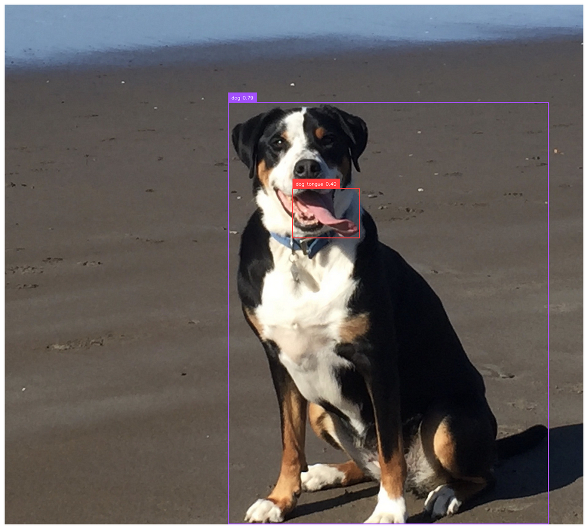
GroundingDINO, for these not acquainted, merges object detection with language permitting customers to produce a immediate like “a tennis participant” which then leads the mannequin to return candidate object detection packing containers that match the outline. RoboFlow has an ideal tutorial right here for these excited about utilizing it — however I’ve pasted some very primary code under as properly. As seen under you’ll be able to immediate the mannequin to determine objects that will very hardly ever if ever be tagged in an object detection dataset like a canine’s tongue!
from groundingdino.util.inference import load_model, load_image, predict, annotateBOX_TRESHOLD = 0.35
TEXT_TRESHOLD = 0.25
# processes the picture to GroundingDino requirements
image_source, picture = load_image("canine.jpg")
immediate = "canine tongue, canine"
packing containers, logits, phrases = predict(
mannequin=mannequin,
picture=picture,
caption=TEXT_PROMPT,
box_threshold=BOX_TRESHOLD,
text_threshold=TEXT_TRESHOLD
)

Nonetheless, distinguishing gamers on knowledgeable tennis court docket isn’t so simple as prompting for “tennis gamers.” The mannequin typically misidentifies different people on the court docket, reminiscent of line judges, ball folks, and different umpires, inflicting jumpy and inconsistent annotations. Moreover, the mannequin typically fails to even detect the gamers in sure frames, resulting in gaps and non-persistent packing containers that don’t reliably seem in every body.

To deal with these challenges, we apply a number of focused strategies. First, we slender down the detection packing containers to simply the highest three chances from all doable packing containers. Typically, line judges have the next chance rating than gamers, which is why we don’t filter to solely two packing containers. Nonetheless, this raises a brand new query: how can we mechanically distinguish gamers from line judges in every body?
We noticed that detection packing containers for line and ball personnel sometimes have shorter time spans, typically lasting only a few frames. Based mostly on this, we hypothesize that by associating packing containers throughout consecutive frames, we might filter out those that solely seem briefly, thereby isolating the gamers.
So how can we obtain this sort of affiliation between objects throughout frames? Luckily, the sector of multi-object monitoring has extensively studied this drawback. Kalman filters are a mainstay in multi-object monitoring, typically mixed with different identification metrics, reminiscent of colour. For our functions, a primary Kalman filter implementation is enough. In easy phrases (for a deeper dive, test this article out), a Kalman filter is a technique for probabilistically estimating an object’s place primarily based on earlier measurements. It’s significantly efficient with noisy knowledge but additionally works properly associating objects throughout time in movies, even when detections are inconsistent reminiscent of when a participant is just not tracked each body. We implement a complete Kalman filter right here however will stroll via a few of the major steps within the following paragraphs.
A Kalman filter state for two dimensions is sort of easy as proven under. All we now have to do is preserve observe of the x and y location in addition to the objects velocity in each instructions (we ignore acceleration).
class KalmanStateVector2D:
x: float
y: float
vx: float
vy: float
The Kalman filter operates in two steps: it first predicts an object’s location within the subsequent body, then updates this prediction primarily based on a brand new measurement — in our case, from the article detector. Nonetheless, in our instance a brand new body might have a number of new objects, or it might even drop objects that have been current within the earlier body resulting in the query of how we will affiliate packing containers we now have seen beforehand with these seen at the moment.
We select to do that through the use of the Mahalanobis distance, coupled with a chi-squared check, to evaluate the chance {that a} present detection matches a previous object. Moreover, we preserve a queue of previous objects so we now have an extended ‘reminiscence’ than only one body. Particularly, our reminiscence shops the trajectory of any object seen over the past 30 frames. Then for every object we discover in a brand new body we iterate over our reminiscence and discover the earlier object probably to be a match with the present given by the chance given from the Mahalanbois distance. Nonetheless, it’s doable we’re seeing a completely new object as properly, wherein case we must always add a brand new object to our reminiscence. If any object has <30% chance of being related to any field in our reminiscence we add it to our reminiscence as a brand new object.
We offer our full Kalman filter under for these preferring code.
from dataclasses import dataclassimport numpy as np
from scipy import stats
class KalmanStateVectorNDAdaptiveQ:
states: np.ndarray # for two dimensions these are [x, y, vx, vy]
cov: np.ndarray # 4x4 covariance matrix
def __init__(self, states: np.ndarray) -> None:
self.state_matrix = states
self.q = np.eye(self.state_matrix.form[0])
self.cov = None
# assumes a single step transition
self.f = np.eye(self.state_matrix.form[0])
# divide by 2 as we now have a velocity for every state
index = self.state_matrix.form[0] // 2
self.f[:index, index:] = np.eye(index)
def initialize_covariance(self, noise_std: float) -> None:
self.cov = np.eye(self.state_matrix.form[0]) * noise_std**2
def predict_next_state(self, dt: float) -> None:
self.state_matrix = self.f @ self.state_matrix
self.predict_next_covariance(dt)
def predict_next_covariance(self, dt: float) -> None:
self.cov = self.f @ self.cov @ self.f.T + self.q
def __add__(self, different: np.ndarray) -> np.ndarray:
return self.state_matrix + different
def update_q(
self, innovation: np.ndarray, kalman_gain: np.ndarray, alpha: float = 0.98
) -> None:
innovation = innovation.reshape(-1, 1)
self.q = (
alpha * self.q
+ (1 - alpha) * kalman_gain @ innovation @ innovation.T @ kalman_gain.T
)
class KalmanNDTrackerAdaptiveQ:
def __init__(
self,
state: KalmanStateVectorNDAdaptiveQ,
R: float, # R
Q: float, # Q
h: np.ndarray = None,
) -> None:
self.state = state
self.state.initialize_covariance(Q)
self.predicted_state = None
self.previous_states = []
self.h = np.eye(self.state.state_matrix.form[0]) if h is None else h
self.R = np.eye(self.h.form[0]) * R**2
self.previous_measurements = []
self.previous_measurements.append(
(self.h @ self.state.state_matrix).reshape(-1, 1)
)
def predict(self, dt: float) -> None:
self.previous_states.append(self.state)
self.state.predict_next_state(dt)
def update_covariance(self, achieve: np.ndarray) -> None:
self.state.cov -= achieve @ self.h @ self.state.cov
def replace(
self, measurement: np.ndarray, dt: float = 1, predict: bool = True
) -> None:
"""Measurement will likely be a x, y place"""
self.previous_measurements.append(measurement)
assert dt == 1, "Solely single step transitions are supported on account of F matrix"
if predict:
self.predict(dt=dt)
innovation = measurement - self.h @ self.state.state_matrix
gain_invertible = self.h @ self.state.cov @ self.h.T + self.R
gain_inverse = np.linalg.inv(gain_invertible)
achieve = self.state.cov @ self.h.T @ gain_inverse
new_state = self.state.state_matrix + achieve @ innovation
self.update_covariance(achieve)
self.state.update_q(innovation, achieve)
self.state.state_matrix = new_state
def compute_mahalanobis_distance(self, measurement: np.ndarray) -> float:
innovation = measurement - self.h @ self.state.state_matrix
return np.sqrt(
innovation.T
@ np.linalg.inv(
self.h @ self.state.cov @ self.h.T + self.R
)
@ innovation
)
def compute_p_value(self, distance: float) -> float:
return 1 - stats.chi2.cdf(distance, df=self.h.form[0])
def compute_p_value_from_measurement(self, measurement: np.ndarray) -> float:
"""Returns the chance that the measurement is in line with the expected state"""
distance = self.compute_mahalanobis_distance(measurement)
return self.compute_p_value(distance)
Having tracked each detected object over the previous 30 frames, we will now devise heuristics to pinpoint which packing containers probably characterize our gamers. We examined two approaches: deciding on the packing containers nearest the middle of the baseline, and selecting these with the longest noticed historical past in our reminiscence. Empirically, the primary technique typically flagged line judges as gamers every time the precise participant moved away from the baseline, making it much less dependable. In the meantime, we seen that GroundingDino tends to “flicker” between totally different line judges and ball folks, whereas real gamers preserve a considerably steady presence. In consequence, our remaining rule is to choose the packing containers in our reminiscence with the longest monitoring historical past because the true gamers. As you’ll be able to see within the preliminary video, it’s surprisingly efficient for such a easy rule!
With our monitoring system now established on the picture, we will transfer towards a extra conventional evaluation by monitoring gamers from a chook’s-eye perspective. This viewpoint permits the analysis of key metrics, reminiscent of complete distance traveled, participant pace, and court docket positioning tendencies. For instance, we might analyze whether or not a participant often targets their opponent’s backhand primarily based on location throughout a degree. To perform this, we have to venture the participant coordinates from the picture onto a standardized court docket template considered from above, aligning the angle for spatial evaluation.
That is the place homography comes into play. Homography describes the mapping between two surfaces, which, in our case, means mapping the factors on our unique picture to an overhead court docket view. By figuring out a number of keypoints within the unique picture — reminiscent of line intersections on a court docket — we will calculate a homography matrix that interprets any level to a chook’s-eye view. To create this homography matrix, we first must determine these ‘keypoints.’ Varied open-source, permissively licensed fashions on platforms like RoboFlow may help detect these factors, or we will label them ourselves on a reference picture to make use of within the transformation.

After labeling these keypoints, the following step is to match them with corresponding factors on a reference court docket picture to generate a homography matrix. Utilizing OpenCV, we will then create this transformation matrix with a number of easy traces of code!
import numpy as np
import cv2# order of the factors issues
supply = np.array(keypoints) # (n, 2) matrix
goal = np.array(court_coords) # (n, 2) matrix
m, _ = cv2.findHomography(supply, goal)
With the homography matrix in hand, we will map any level from our picture onto the reference court docket. For this venture, our focus is on the participant’s place on the court docket. To find out this, we take the midpoint on the base of every participant’s bounding field, utilizing it as their location on the court docket within the chook’s-eye view.
In abstract, this venture demonstrates how we will use GroundingDINO’s zero-shot capabilities to trace tennis gamers with out counting on labeled knowledge, reworking complicated object detection into actionable participant monitoring. By tackling key challenges — reminiscent of distinguishing gamers from different on-court personnel, making certain constant monitoring throughout frames, and mapping participant actions to a chook’s-eye view of the court docket — we’ve laid the groundwork for a strong monitoring pipeline all with out the necessity for express labels.
This method doesn’t simply unlock insights like distance traveled, pace, and positioning but additionally opens the door to deeper match analytics, reminiscent of shot concentrating on and strategic court docket protection. With additional refinement, together with distilling a YOLO or RT-DETR mannequin from GroundingDINO outputs, we might even develop a real-time monitoring system that rivals current business options, offering a strong software for each teaching and fan engagement on this planet of tennis.


