


to be the state-of-the-art object detection algorithm, seemed to develop into out of date due to the looks of different strategies like SSD (Single Shot Multibox Detector), DSSD (Deconvolutional Single Shot Detector), and RetinaNet. Lastly, after two years because the introduction of YOLOv2, the authors determined to enhance the algorithm the place they finally got here up with the following YOLO model reported in a paper titled “YOLOv3: An Incremental Enchancment” [1]. Because the title suggests, there have been certainly not many issues the authors improved upon YOLOv2 when it comes to the underlying algorithm. However hey, on the subject of efficiency, it really appears fairly spectacular.
On this article I’m going to speak in regards to the modifications the authors made to YOLOv2 to create YOLOv3 and the way to implement the mannequin structure from scratch with PyTorch. I extremely suggest you studying my earlier article about YOLOv1 [2, 3] and YOLOv2 [4] earlier than this one, except you already obtained a powerful basis in how these two earlier variations of YOLO work.
What Makes YOLOv3 Higher Than YOLOv2
The Vanilla Darknet-53
The modification the authors made was primarily associated to the structure, by which they proposed a spine mannequin known as Darknet-53. See the detailed construction of this community in Determine 1. Because the title suggests, this mannequin is an enchancment upon the Darknet-19 utilized in YOLOv2. In the event you rely the variety of layers in Darknet-53, you will discover that this community consists of 52 convolution layers and a single fully-connected layer on the finish. Remember that later once we implement it on YOLOv3, we’ll feed it with pictures of measurement 416×416 fairly than 256×256 as written within the determine.
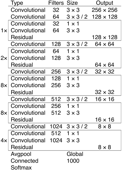
In the event you’re aware of Darknet-19, you need to keep in mind that it performs spatial downsmapling utilizing maxpooling operations after each stack of a number of convolution layers. In Darknet-53, authors changed these pooling operations with convolutions of stride 2. This was primarily executed as a result of maxpooling layer fully ignores non-maximum numbers, inflicting us to lose a variety of info contained within the decrease depth pixels. We will really use average-pooling instead, however in principle, this method received’t be optimum both as a result of all pixels throughout the small area are weighted the identical. In order an answer, authors determined to make use of convolution layer with a stride of two, which by doing so the mannequin will be capable of cut back picture decision whereas capturing spatial info with particular weightings. You may see the illustration for this in Determine 2 beneath.

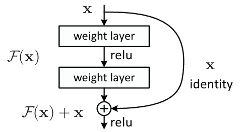
Subsequent, the spine of this YOLO model is now outfitted with residual blocks which the thought is originated from ResNet. One factor that I wish to emphasize relating to our implementation is the activation operate throughout the residual block. You may see in Determine 3 beneath that based on the unique ResNet paper, the second activation operate is positioned after the element-wise summation. Nevertheless, primarily based on the opposite tutorials that I learn [6, 7], I discovered that within the case of YOLOv3 the second activation operate is positioned proper after the load layer as an alternative (earlier than summation). So later within the implementation, I made a decision to comply with the information in these tutorials because the YOLOv3 paper doesn’t give any explanations about it.
Darknet-53 With Detection Heads
Remember that the structure in Determine 1 is just meant for classification. Thus, we have to change all the pieces after the final residual block if we wish to make it suitable for detection duties. Once more, the unique YOLOv3 paper additionally doesn’t present the detailed implementation information, therefore I made a decision to seek for it and finally obtained one from the paper referenced as [9]. I redraw the illustration from that paper to make the structure appears clearer as proven in Determine 4 beneath.

There are literally a lot of issues to clarify relating to the above structure. Now let’s begin from the half I confer with because the detection heads. Totally different from the earlier YOLO variations which relied on a single head, right here in YOLOv3 we have now 2 extra heads. Thus, we’ll later have 3 prediction tensors for each single enter picture. These three detection heads have completely different specializations: the leftmost head (13×13) is the one accountable to detect massive objects, the center head (26×26) is for detecting medium-sized objects, and the one on the appropriate (52×52) is used to detect objects of small measurement. We will consider the 52×52 tensor because the characteristic map that comprises the detailed illustration of a picture, therefore is appropriate to detect small objects. Conversely, the 13×13 prediction tensor is supposed to detect massive objects due to its decrease spatial decision which is efficient at capturing the final form of an object.
Nonetheless with the detection head, you may also see in Determine 4 that the three prediction tensors have 255 channels. To grasp the place this quantity comes from, we first must know that every detection head has 3 prior packing containers. Following the rule given in YOLOv2, every of those prior packing containers is configured such that it could possibly predict its personal object class independently. With this mechanism, the characteristic vector of every grid cell may be obtained by computing B×(5+C), the place B is the variety of prior packing containers, C is the variety of object courses, and 5 is the xywh and the bounding field confidence (a.ok.a. objectness). Within the case of YOLOv3, every detection head has 3 prior packing containers and 80 courses, assuming that we prepare it on 80-class COCO dataset. By plugging these numbers to the formulation, we receive 3×(5+80)=255 prediction values for a single grid cell.
The truth is, utilizing multi-head mechanism like this permits the mannequin to detect extra objects as in comparison with the sooner YOLO variations. Beforehand in YOLOv1, since a picture is split into 7×7 grid cells and every of these can predict 2 bounding packing containers, therefore there are 98 objects potential to be detected. In the meantime in YOLOv2, a picture is split into 13×13 grid cells by which a single cell is able to producing 5 bounding packing containers, making YOLOv2 capable of detect as much as 845 objects inside a single picture. This primarily permits YOLOv2 to have a greater recall than YOLOv1. In principle, YOLOv3 is probably capable of obtain an excellent larger recall, particularly when examined on a picture that comprises a variety of objects due to the bigger variety of potential detections. We will calculate the variety of most bounding packing containers for a single picture in YOLOv3 by computing (13×13×3) + (26×26×3) + (52×52×3) = 507 + 2028 + 8112 = 10647, the place 13×13, 26×26, and 52×25 are the variety of grid cells inside every prediction tensor, whereas 3 is the variety of prior packing containers a single grid cell has.
We will additionally see in Determine 4 that there are two concatenation steps integrated within the community, i.e., between the unique Darknet-53 structure and the detection heads. The target of those steps is to mix info from the deeper layer with the one from the shallower layer. Combining info from completely different depths like that is necessary as a result of on the subject of detecting smaller objects, we do want each an in depth spatial info (contained within the shallower layer) and a greater semantic info (contained within the deeper layer). Remember that the characteristic map from the deeper layer has a smaller spatial dimension, therefore we have to broaden it earlier than really doing the concatenation. That is primarily the rationale that we have to place an upsampling layer proper earlier than we do the concatenation.
Multi-Label Classification
Aside from the structure, the authors additionally modified the category labeling mechanism. As an alternative of utilizing a typical multiclass classification paradigm, they proposed to make use of the so-called multilabel classification. In the event you’re not but aware of it, that is mainly a way the place a picture may be assigned a number of labels without delay. Check out Determine 5 beneath to higher perceive this concept. On this instance, the picture on the left belongs to the category particular person, athlete, runner, and man concurrently. In a while, YOLOv3 can also be anticipated to have the ability to make a number of class predictions on the identical detected object.

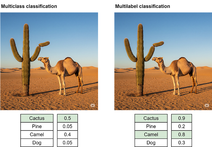
To ensure that the mannequin to foretell a number of labels, we have to deal with every class prediction output as an unbiased binary classifier. Have a look at Determine 6 beneath to see how multiclass classification differs from multilabel classification. The illustration on the left is a situation once we use a typical multiclass classification mechanism. Right here you’ll be able to see that the possibilities of all courses sum to 1 due to the character of the softmax activation operate throughout the output layer. On this instance, because the class camel is predicted with the very best chance, then the ultimate prediction can be camel no matter how excessive the prediction confidence of the opposite courses is.
Then again, if we use multilabel classification, there’s a chance that the sum of all class prediction possibilities is larger than 1 as a result of we use sigmoid activation operate which by nature doesn’t limit the sum of all prediction confidence scores to 1. Because of this purpose, later within the implementation we will merely apply a particular threshold to contemplate a category predicted. Within the instance beneath, if we assume that the brink is 0.7, then the picture can be predicted as each cactus and camel.
Modified Loss Perform
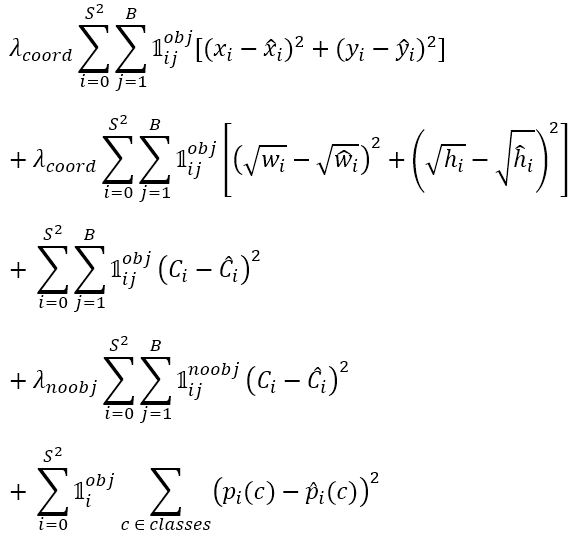
One other modification the authors made was associated to the loss operate. Now take a look at the loss operate of YOLOv1 in Determine 7 beneath. As a refresher, the first and 2nd rows are accountable to compute the bounding field loss, the third and 4th rows are for the objectness confidence loss, and the fifth row is for computing the classification loss. Do not forget that in YOLOv1 the authors used SSE (Sum of Squared Errors) in all these 5 rows to make issues easy.
In YOLOv3, the authors determined to interchange the objectness loss (the third and 4th rows) with binary cross entropy, contemplating that the predictions similar to this half is just both 1 or 0, i.e., whether or not there’s an object midpoint or not. Thus, it makes extra sense to deal with this as a binary classification fairly than a regression drawback.
Binary cross entropy may also be used within the classification loss (fifth row). That is primarily as a result of we use multilabel classification mechanism we mentioned earlier, the place we deal with every of the output neuron as an unbiased binary classifier. Do not forget that if we have been to carry out a typical classification job, we usually must set the loss operate to categorical cross entropy as an alternative.
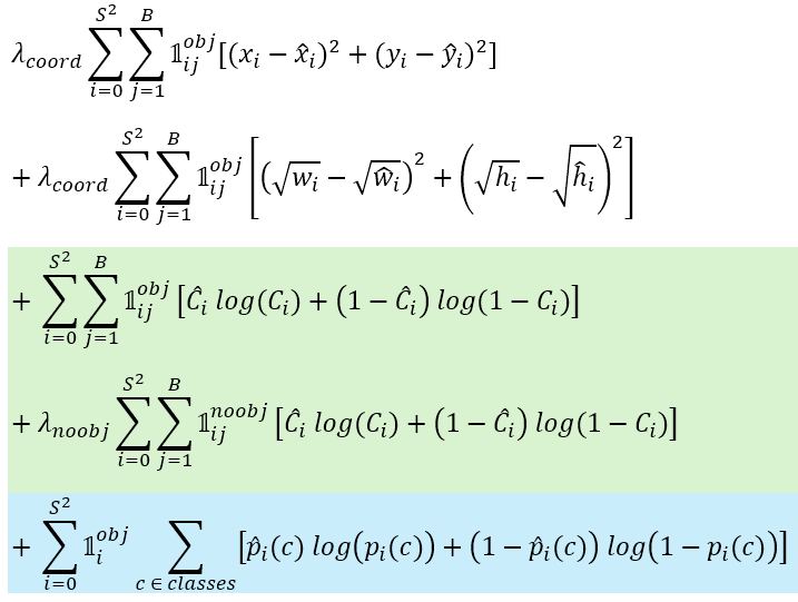
Now beneath is what the loss operate appears like after we change the SSE with binary cross entropy for the objectness (inexperienced) and the multilabel classification (blue) components. Word that this equation is created primarily based on the YouTube tutorial I watched given at reference quantity [12] as a result of, once more, the authors don’t explicitly present the ultimate loss operate within the paper.
Some Experimental Outcomes
With all of the modifications mentioned above, the authors discovered that the development in efficiency is fairly spectacular. The primary experimental outcome I wish to present you is said to the efficiency of the spine mannequin in classifying pictures on ImageNet dataset. You may see in Determine 9 beneath that the development from Darknet-19 (YOLOv2) to Darknet-53 (YOLOv3) is sort of vital when it comes to each the top-1 accuracy (74.1 to 77.2) and the top-5 accuracy (91.8 to 93.8). It’s essential to acknowledge that ResNet-101 and ResNet-152 certainly additionally carry out pretty much as good as Darknet-53 in accuracy, but when we examine the FPS (measured on Nvidia Titan X), we will see that Darknet-53 is lots sooner than each ResNet variants.

The same conduct is also noticed on object detection job, the place it’s seen in Determine 10 that every one YOLOv3 variants efficiently obtained the quickest computation time amongst all different strategies regardless of not having the perfect accuracy. You may see within the determine that the biggest YOLOv3 variant is sort of 4 instances sooner than the biggest RetinaNet variant (51 ms vs 198 ms). Furthermore, the biggest YOLOv3 variant itself already surpasses the mAP of the smallest RetinaNet variant (33.0 vs 32.5) whereas nonetheless having a sooner inference time (51 ms vs 73 ms). These experimental outcomes primarily show that YOLOv3 grew to become the state-of-the-art object detection mannequin when it comes to computational pace at that second.

YOLOv3 Structure Implementation
As we have now already mentioned just about all the pieces in regards to the principle behind YOLOv3, we will now begin implementing the structure from scratch. In Codeblock 1 beneath, I import the torch module and its nn submodule. Right here I additionally initialize the NUM_PRIORS and NUM_CLASS variables, by which these two correspond to the variety of prior packing containers inside every grid cell and the variety of object courses within the dataset, respectively.
# Codeblock 1
import torch
import torch.nn as nn

NUM_PRIORS = 3
NUM_CLASS  = 80
Convolutional Block Implementation
What I’m going to implement first is the principle constructing block of the community, which I confer with because the Convolutional block as seen in Codeblock 2. The construction of this block is sort of a bit the identical because the one utilized in YOLOv2, the place it follows the Conv-BN-Leaky ReLU sample. After we use this type of construction, don’t neglect to set the bias parameter of the conv layer to False (at line #(1)) as a result of utilizing bias time period is considerably ineffective if we instantly place a batch normalization layer proper after it. Right here I additionally configure the padding of the conv layer such that it’ll robotically set to 1 at any time when the kernel measurement is 3×3 or 0 at any time when we use 1×1 kernel (#(2)). Subsequent, because the conv, bn, and leaky_relu have been initialized, we will merely join all of them utilizing the code written contained in the ahead() technique (#(3)).
# Codeblock 2
class Convolutional(nn.Module):
    def __init__(self,
                 in_channels,
                 out_channels,
                 kernel_size,
                 stride=1):
        tremendous().__init__()

        self.conv = nn.Conv2d(in_channels=in_channels,
                              out_channels=out_channels,
                              kernel_size=kernel_size,
                              stride=stride,
                              bias=False,                            #(1)
                              padding=1 if kernel_size==3 else 0)    #(2)

        self.bn = nn.BatchNorm2d(num_features=out_channels)

        self.leaky_relu = nn.LeakyReLU(negative_slope=0.1)

    def ahead(self, x):        #(3)
        print(f'originalt: {x.measurement()}')

        x = self.conv(x)
        print(f'after convt: {x.measurement()}')

        x = self.bn(x)
        print(f'after bnt: {x.measurement()}')

        x = self.leaky_relu(x)
        print(f'after leaky relu: {x.measurement()}')

        return x
We simply wish to be certain that our major constructing block is working correctly, we’ll take a look at it by simulating the very first Convolutional block in Determine 1. Do not forget that since YOLOv3 takes a picture of measurement 416×416 because the enter, right here in Codeblock 3 I create a dummy tensor of that form to simulate a picture handed by way of that layer. Additionally, observe that right here I depart the stride to the default (1) as a result of at this level we don’t wish to carry out spatial downsampling.
# Codeblock 3
convolutional = Convolutional(in_channels=3,
                              out_channels=32,
                              kernel_size=3)

x = torch.randn(1, 3, 416, 416)
out = convolutional(x)
# Codeblock 3 Output
unique : torch.Dimension([1, 3, 416, 416])
after conv : torch.Dimension([1, 32, 416, 416])
after bn : torch.Dimension([1, 32, 416, 416])
after leaky relu : torch.Dimension([1, 32, 416, 416])Now let’s take a look at our Convolutional block once more, however this time I’ll set the stride to 2 to simulate the second convolutional block within the structure. We will see within the output beneath that the spatial dimension halves from 416×416 to 208×208, indicating that this method is a legitimate substitute for the maxpooling layers we beforehand had in YOLOv1 and YOLOv2.
# Codeblock 4
convolutional = Convolutional(in_channels=32,
                              out_channels=64,
                              kernel_size=3,
                              stride=2)

x = torch.randn(1, 32, 416, 416)
out = convolutional(x)
# Codeblock 4 Output
unique : torch.Dimension([1, 32, 416, 416])
after conv : torch.Dimension([1, 64, 208, 208])
after bn : torch.Dimension([1, 64, 208, 208])
after leaky relu : torch.Dimension([1, 64, 208, 208])Residual Block Implementation
Because the Convolutional block is completed, what I’m going to do now’s to implement the following constructing block: Residual. This block usually follows the construction I displayed again in Determine 3, the place it consists of a residual connection that skips by way of two Convolutional blocks. Check out the Codeblock 5 beneath to see how I implement it.
The 2 convolution layers themselves comply with the sample in Determine 1, the place the primary Convolutional halves the variety of channels (#(1)) which is able to then be doubled once more by the second Convolutional (#(3)). Right here you additionally want to notice that the primary convolution makes use of 1×1 kernel (#(2)) whereas the second makes use of 3×3 (#(4)). Subsequent, what we do contained in the ahead() technique is solely connecting the 2 convolutions sequentially, which the ultimate output is summed with the unique enter tensor (#(5)) earlier than being returned.
# Codeblock 5
class Residual(nn.Module):
    def __init__(self, num_channels):
        tremendous().__init__()
        self.conv0 = Convolutional(in_channels=num_channels,
                                   out_channels=num_channels//2,   #(1)
                                   kernel_size=1,       #(2)
                                   stride=1)

        self.conv1 = Convolutional(in_channels=num_channels//2,
                                   out_channels=num_channels,      #(3)
                                   kernel_size=3,       #(4)
                                   stride=1)

    def ahead(self, x):
        unique = x.clone()
        print(f'originalt: {x.measurement()}')

        x = self.conv0(x)
        print(f'after conv0t: {x.measurement()}')

        x = self.conv1(x)
        print(f'after conv1t: {x.measurement()}')

        x = x + unique      #(5)
        print(f'after summationt: {x.measurement()}')

        return x
We are going to now take a look at the Residual block we simply created utilizing the Codeblock 6 beneath. Right here I set the num_channels parameter to 64 as a result of I wish to simulate the very first residual block within the Darknet-53 structure (see Determine 1).
# Codeblock 6
residual = Residual(num_channels=64)

x = torch.randn(1, 64, 208, 208)
out = residual(x)
# Codeblock 6 Output
unique : torch.Dimension([1, 64, 208, 208])
after conv0 : torch.Dimension([1, 32, 208, 208])
after conv1 : torch.Dimension([1, 64, 208, 208])
after summation : torch.Dimension([1, 64, 208, 208])In the event you take a more in-depth take a look at the above output, you’ll discover that the form of the enter and output tensors are precisely the identical. This primarily permits us to repeat a number of residual blocks simply. Within the Codeblock 7 beneath I attempt to stack 4 residual blocks and go a tensor by way of it, simulating the final stack of residual blocks within the structure.
# Codeblock 7
residuals = nn.ModuleList([])
for _ in vary(4):
    residual = Residual(num_channels=1024)
    residuals.append(residual)

x = torch.randn(1, 1024, 13, 13)

for i in vary(len(residuals)):
    x = residuals[i](x)
    print(f'after residuals #{i}t: {x.measurement()}')
# Codeblock 7 Output
after residuals #0 : torch.Dimension([1, 1024, 13, 13])
after residuals #1 : torch.Dimension([1, 1024, 13, 13])
after residuals #2 : torch.Dimension([1, 1024, 13, 13])
after residuals #3 : torch.Dimension([1, 1024, 13, 13])Darknet-53 Implementation
Utilizing the Convolutional and Residual constructing blocks we created earlier, we will now really assemble the Darknet-53 mannequin. All the pieces I initialize contained in the __init__() technique beneath relies on the structure in Determine 1. Nevertheless, keep in mind that we have to cease on the final residual block since we don’t want the worldwide common pooling and the fully-connected layers. Not solely that, on the strains marked with #(1) and #(2) I retailer the intermediate characteristic maps in separate variables (branch0 and branch1). We are going to later return these characteristic maps alongside the output from the principle circulate (x) (#(3)) to implement the branches that circulate into the three detection heads.
# Codeblock 8
class Darknet53(nn.Module):
    def __init__(self):
        tremendous().__init__()

        self.convolutional0 = Convolutional(in_channels=3,
                                            out_channels=32,
                                            kernel_size=3)

        self.convolutional1 = Convolutional(in_channels=32,
                                            out_channels=64,
                                            kernel_size=3,
                                            stride=2)

        self.residuals0 = nn.ModuleList([Residual(num_channels=64) for _ in range(1)])

        self.convolutional2 = Convolutional(in_channels=64,
                                            out_channels=128,
                                            kernel_size=3,
                                            stride=2)

        self.residuals1 = nn.ModuleList([Residual(num_channels=128) for _ in range(2)])

        self.convolutional3 = Convolutional(in_channels=128,
                                            out_channels=256,
                                            kernel_size=3,
                                            stride=2)

        self.residuals2 = nn.ModuleList([Residual(num_channels=256) for _ in range(8)])

        self.convolutional4 = Convolutional(in_channels=256,
                                            out_channels=512,
                                            kernel_size=3,
                                            stride=2)

        self.residuals3 = nn.ModuleList([Residual(num_channels=512) for _ in range(8)])

        self.convolutional5 = Convolutional(in_channels=512,
                                            out_channels=1024,
                                            kernel_size=3,
                                            stride=2)

        self.residuals4 = nn.ModuleList([Residual(num_channels=1024) for _ in range(4)])

    def ahead(self, x):
        print(f'originaltt: {x.measurement()}n')

        x = self.convolutional0(x)
        print(f'after convolutional0t: {x.measurement()}')

        x = self.convolutional1(x)
        print(f'after convolutional1t: {x.measurement()}n')

        for i in vary(len(self.residuals0)):
            x = self.residuals0[i](x)
            print(f'after residuals0 #{i}t: {x.measurement()}')

        x = self.convolutional2(x)
        print(f'nafter convolutional2t: {x.measurement()}n')

        for i in vary(len(self.residuals1)):
            x = self.residuals1[i](x)
            print(f'after residuals1 #{i}t: {x.measurement()}')

        x = self.convolutional3(x)
        print(f'nafter convolutional3t: {x.measurement()}n')

        for i in vary(len(self.residuals2)):
            x = self.residuals2[i](x)
            print(f'after residuals2 #{i}t: {x.measurement()}')

        branch0 = x.clone()           #(1)

        x = self.convolutional4(x)
        print(f'nafter convolutional4t: {x.measurement()}n')

        for i in vary(len(self.residuals3)):
            x = self.residuals3[i](x)
            print(f'after residuals3 #{i}t: {x.measurement()}')

        branch1 = x.clone()           #(2)

        x = self.convolutional5(x)
        print(f'nafter convolutional5t: {x.measurement()}n')

        for i in vary(len(self.residuals4)):
            x = self.residuals4[i](x)
            print(f'after residuals4 #{i}t: {x.measurement()}')

        return branch0, branch1, x    #(3)
Now we take a look at our Darknet53 class by operating the Codeblock 9 beneath. You may see within the ensuing output that all the pieces appears to work correctly as the form of the tensor appropriately transforms based on the information in Determine 1. One factor that I haven’t talked about earlier than is that this Darknet-53 structure downscales the enter picture by an element of 32. So, with this downsampling issue, an enter picture of form 256×256 will develop into 8×8 in the long run (as proven in Determine 1), whereas an enter of form 416×416 will lead to a 13×13 prediction tensor.
# Codeblock 9
darknet53 = Darknet53()

x = torch.randn(1, 3, 416, 416)
out = darknet53(x)
# Codeblock 9 Output
unique : torch.Dimension([1, 3, 416, 416])
after convolutional0 : torch.Dimension([1, 32, 416, 416])
after convolutional1 : torch.Dimension([1, 64, 208, 208])
after residuals0 #0 : torch.Dimension([1, 64, 208, 208])
after convolutional2 : torch.Dimension([1, 128, 104, 104])
after residuals1 #0 : torch.Dimension([1, 128, 104, 104])
after residuals1 #1 : torch.Dimension([1, 128, 104, 104])
after convolutional3 : torch.Dimension([1, 256, 52, 52])
after residuals2 #0 : torch.Dimension([1, 256, 52, 52])
after residuals2 #1 : torch.Dimension([1, 256, 52, 52])
after residuals2 #2 : torch.Dimension([1, 256, 52, 52])
after residuals2 #3 : torch.Dimension([1, 256, 52, 52])
after residuals2 #4 : torch.Dimension([1, 256, 52, 52])
after residuals2 #5 : torch.Dimension([1, 256, 52, 52])
after residuals2 #6 : torch.Dimension([1, 256, 52, 52])
after residuals2 #7 : torch.Dimension([1, 256, 52, 52])
after convolutional4 : torch.Dimension([1, 512, 26, 26])
after residuals3 #0 : torch.Dimension([1, 512, 26, 26])
after residuals3 #1 : torch.Dimension([1, 512, 26, 26])
after residuals3 #2 : torch.Dimension([1, 512, 26, 26])
after residuals3 #3 : torch.Dimension([1, 512, 26, 26])
after residuals3 #4 : torch.Dimension([1, 512, 26, 26])
after residuals3 #5 : torch.Dimension([1, 512, 26, 26])
after residuals3 #6 : torch.Dimension([1, 512, 26, 26])
after residuals3 #7 : torch.Dimension([1, 512, 26, 26])
after convolutional5 : torch.Dimension([1, 1024, 13, 13])
after residuals4 #0 : torch.Dimension([1, 1024, 13, 13])
after residuals4 #1 : torch.Dimension([1, 1024, 13, 13])
after residuals4 #2 : torch.Dimension([1, 1024, 13, 13])
after residuals4 #3 : torch.Dimension([1, 1024, 13, 13])At this level we will additionally see what the outputs produced by the three branches appear to be just by printing out the shapes of branch0, branch1, and x as proven in Codeblock 10 beneath. Discover that the spatial dimensions of those three tensors fluctuate. In a while, the tensors from the deeper layers can be upsampled in order that we will carry out channel-wise concatenation with these from the shallower ones.
# Codeblock 10
print(out[0].form)      # branch0
print(out[1].form)      # branch1
print(out[2].form)      # x
# Codeblock 10 Output
torch.Dimension([1, 256, 52, 52])
torch.Dimension([1, 512, 26, 26])
torch.Dimension([1, 1024, 13, 13])Detection Head Implementation
In the event you return to Determine 4, you’ll discover that every of the detection heads consists of two convolution layers. Nevertheless, these two convolutions are usually not equivalent. In Codeblock 11 beneath I take advantage of the Convolutional block for the primary one and the plain nn.Conv2d for the second. That is primarily executed as a result of the second convolution acts as the ultimate layer, therefore is answerable for giving uncooked output (as an alternative of being normalized and ReLU-ed).
# Codeblock 11
class DetectionHead(nn.Module):
    def __init__(self, num_channels):
        tremendous().__init__()

        self.convhead0 = Convolutional(in_channels=num_channels,
                                       out_channels=num_channels*2,
                                       kernel_size=3)

        self.convhead1 = nn.Conv2d(in_channels=num_channels*2,
                                   out_channels=NUM_PRIORS*(NUM_CLASS+5),
                                   kernel_size=1)

    def ahead(self, x):
        print(f'originalt: {x.measurement()}')

        x = self.convhead0(x)
        print(f'after convhead0t: {x.measurement()}')

        x = self.convhead1(x)
        print(f'after convhead1t: {x.measurement()}')

        return x
Now in Codeblock 12 I’ll attempt to simulate the 13×13 detection head, therefore I set the enter characteristic map to have the form of 512×13×13 (#(1)). By the way in which you’ll know the place the quantity 512 comes from later within the subsequent part.
# Codeblock 12
detectionhead = DetectionHead(num_channels=512)

x = torch.randn(1, 512, 13, 13)    #(1)
out = detectionhead(x)
And beneath is what the ensuing output appears like. We will see right here that the tensor expands to 1024×13×13 earlier than finally shrink to 255×13×13. Do not forget that in YOLOv3 so long as we set NUM_PRIORS to three and NUM_CLASS to 80, the variety of output channel will all the time be 255 whatever the variety of enter channel fed into the DetectionHead.
# Codeblock 12 Output
unique        : torch.Dimension([1, 512, 13, 13])
after convhead0 : torch.Dimension([1, 1024, 13, 13])
after convhead1 : torch.Dimension([1, 255, 13, 13])
The Total YOLOv3 Structure
Okay now — since we have now initialized the principle constructing blocks, what we have to do subsequent is to assemble the complete YOLOv3 structure. Right here I may also talk about the remaining elements we haven’t lined. The code is sort of lengthy although, so I break it down into two codeblocks: Codeblock 13a and Codeblock 13b. Simply be certain that these two codeblocks are written throughout the identical pocket book cell if you wish to run it by yourself.
In Codeblock 13a beneath, what we do first is to initialize the spine mannequin (#(1)). Subsequent, we create a stack of 5 Convolutional blocks which alternately halves and doubles the variety of channels. The conv block that reduces the channel rely makes use of 1×1 kernel whereas the one which will increase it makes use of 3×3 kernel, similar to the construction we use within the Residual block. We initialize this stack of 5 convolutions for the three detection heads. Particularly for the characteristic maps that circulate into the 26×26 and 52×52 heads, we have to initialize one other convolution layer (#(2) and #(4)) and an upsampling layer (#(3) and #(5)) along with the 5 convolutions.
# Codeblock 13a
class YOLOv3(nn.Module):
    def __init__(self):
        tremendous().__init__()

        ###############################################
        # Spine initialization.

        self.darknet53 = Darknet53()    #(1)


        ###############################################
        # For 13x13 output.

        self.conv0  = Convolutional(in_channels=1024, out_channels=512, kernel_size=1)
        self.conv1  = Convolutional(in_channels=512, out_channels=1024, kernel_size=3)
        self.conv2  = Convolutional(in_channels=1024, out_channels=512, kernel_size=1)
        self.conv3  = Convolutional(in_channels=512, out_channels=1024, kernel_size=3)
        self.conv4  = Convolutional(in_channels=1024, out_channels=512, kernel_size=1)

        self.detection_head_large_obj = DetectionHead(num_channels=512)


        ###############################################
        # For 26x26 output.

        self.conv5  = Convolutional(in_channels=512, out_channels=256, kernel_size=1)  #(2)
        self.upsample0 = nn.Upsample(scale_factor=2)      #(3)

        self.conv6  = Convolutional(in_channels=768, out_channels=256, kernel_size=1)
        self.conv7  = Convolutional(in_channels=256, out_channels=512, kernel_size=3)
        self.conv8  = Convolutional(in_channels=512, out_channels=256, kernel_size=1)
        self.conv9  = Convolutional(in_channels=256, out_channels=512, kernel_size=3)
        self.conv10 = Convolutional(in_channels=512, out_channels=256, kernel_size=1)

        self.detection_head_medium_obj = DetectionHead(num_channels=256)


        ###############################################
        # For 52x52 output.

        self.conv11  = Convolutional(in_channels=256, out_channels=128, kernel_size=1)  #(4)
        self.upsample1 = nn.Upsample(scale_factor=2)      #(5)

        self.conv12  = Convolutional(in_channels=384, out_channels=128, kernel_size=1)
        self.conv13  = Convolutional(in_channels=128, out_channels=256, kernel_size=3)
        self.conv14  = Convolutional(in_channels=256, out_channels=128, kernel_size=1)
        self.conv15  = Convolutional(in_channels=128, out_channels=256, kernel_size=3)
        self.conv16  = Convolutional(in_channels=256, out_channels=128, kernel_size=1)

        self.detection_head_small_obj = DetectionHead(num_channels=128)
Now in Codeblock 13b we outline the circulate of the community contained in the ahead() technique. Right here we first go the enter tensor by way of the darknet53 mannequin (#(1)), which produces 3 output tensors: branch0, branch1, and x. Then, what we do subsequent is to attach the layers one after one other based on the circulate given in Determine 4.
# Codeblock 13b
    def ahead(self, x):

        ###############################################
        # Spine.
        branch0, branch1, x = self.darknet53(x)      #(1)
        print(f'branch0ttt: {branch0.measurement()}')
        print(f'branch1ttt: {branch1.measurement()}')
        print(f'xttt: {x.measurement()}n')


        ###############################################
        # Move to 13x13 detection head.

        x = self.conv0(x)
        print(f'after conv0tt: {x.measurement()}')

        x = self.conv1(x)
        print(f'after conv1tt: {x.measurement()}')

        x = self.conv2(x)
        print(f'after conv2tt: {x.measurement()}')

        x = self.conv3(x)
        print(f'after conv3tt: {x.measurement()}')

        x = self.conv4(x)
        print(f'after conv4tt: {x.measurement()}')

        large_obj = self.detection_head_large_obj(x)
        print(f'massive object detectiont: {large_obj.measurement()}n')


        ###############################################
        # Move to 26x26 detection head.

        x = self.conv5(x)
        print(f'after conv5tt: {x.measurement()}')

        x = self.upsample0(x)
        print(f'after upsample0tt: {x.measurement()}')

        x = torch.cat([x, branch1], dim=1)
        print(f'after concatenatet: {x.measurement()}')

        x = self.conv6(x)
        print(f'after conv6tt: {x.measurement()}')

        x = self.conv7(x)
        print(f'after conv7tt: {x.measurement()}')

        x = self.conv8(x)
        print(f'after conv8tt: {x.measurement()}')

        x = self.conv9(x)
        print(f'after conv9tt: {x.measurement()}')

        x = self.conv10(x)
        print(f'after conv10tt: {x.measurement()}')

        medium_obj = self.detection_head_medium_obj(x)
        print(f'medium object detectiont: {medium_obj.measurement()}n')


        ###############################################
        # Move to 52x52 detection head.

        x = self.conv11(x)
        print(f'after conv11tt: {x.measurement()}')

        x = self.upsample1(x)
        print(f'after upsample1tt: {x.measurement()}')

        x = torch.cat([x, branch0], dim=1)
        print(f'after concatenatet: {x.measurement()}')

        x = self.conv12(x)
        print(f'after conv12tt: {x.measurement()}')

        x = self.conv13(x)
        print(f'after conv13tt: {x.measurement()}')

        x = self.conv14(x)
        print(f'after conv14tt: {x.measurement()}')

        x = self.conv15(x)
        print(f'after conv15tt: {x.measurement()}')

        x = self.conv16(x)
        print(f'after conv16tt: {x.measurement()}')

        small_obj = self.detection_head_small_obj(x)
        print(f'small object detectiont: {small_obj.measurement()}n')


        ###############################################
        # Return prediction tensors.

        return large_obj, medium_obj, small_obj
As we have now accomplished the ahead() technique, we will now take a look at the complete YOLOv3 mannequin by passing a single RGB picture of measurement 416×416 as proven in Codeblock 14.
# Codeblock 14
yolov3 = YOLOv3()

x = torch.randn(1, 3, 416, 416)
out = yolov3(x)
Under is what the output appears like after you run the codeblock above. Right here we will see that all the pieces appears to work correctly because the dummy picture efficiently handed by way of all layers within the community. One factor that you just would possibly most likely must know is that the 768-channel characteristic map at line #(4) is obtained from the concatenation between the tensor at strains #(2) and #(3). The same factor additionally applies to the 384-channel tensor at line #(6), by which it’s the concatenation between the characteristic maps at strains #(1) and #(5).
# Codeblock 14 Output
branch0                 : torch.Dimension([1, 256, 52, 52])    #(1)
branch1                 : torch.Dimension([1, 512, 26, 26])    #(2)
x                       : torch.Dimension([1, 1024, 13, 13])

after conv0             : torch.Dimension([1, 512, 13, 13])
after conv1             : torch.Dimension([1, 1024, 13, 13])
after conv2             : torch.Dimension([1, 512, 13, 13])
after conv3             : torch.Dimension([1, 1024, 13, 13])
after conv4             : torch.Dimension([1, 512, 13, 13])
massive object detection  : torch.Dimension([1, 255, 13, 13])

after conv5             : torch.Dimension([1, 256, 13, 13])
after upsample0         : torch.Dimension([1, 256, 26, 26])    #(3)
after concatenate       : torch.Dimension([1, 768, 26, 26])    #(4)
after conv6             : torch.Dimension([1, 256, 26, 26])
after conv7             : torch.Dimension([1, 512, 26, 26])
after conv8             : torch.Dimension([1, 256, 26, 26])
after conv9             : torch.Dimension([1, 512, 26, 26])
after conv10            : torch.Dimension([1, 256, 26, 26])
medium object detection : torch.Dimension([1, 255, 26, 26])

after conv11            : torch.Dimension([1, 128, 26, 26])
after upsample1         : torch.Dimension([1, 128, 52, 52])    #(5)
after concatenate       : torch.Dimension([1, 384, 52, 52])    #(6)
after conv12            : torch.Dimension([1, 128, 52, 52])
after conv13            : torch.Dimension([1, 256, 52, 52])
after conv14            : torch.Dimension([1, 128, 52, 52])
after conv15            : torch.Dimension([1, 256, 52, 52])
after conv16            : torch.Dimension([1, 128, 52, 52])
small object detection  : torch.Dimension([1, 255, 52, 52])
And simply to make issues clearer right here I additionally print out the output of every detection head in Codeblock 15 beneath. We will see right here that every one the ensuing prediction tensors have the form that we anticipated earlier. Thus, I consider our YOLOv3 implementation is appropriate and therefore prepared to coach.
# Codeblock 15
print(out[0].form)
print(out[1].form)
print(out[2].form)
# Codeblock 15 Output
torch.Dimension([1, 255, 13, 13])
torch.Dimension([1, 255, 26, 26])
torch.Dimension([1, 255, 52, 52])I feel that’s just about all the pieces about YOLOv3 and its structure implementation from scratch. As we’ve seen above, the authors efficiently made a formidable enchancment in efficiency in comparison with the earlier YOLO model, though the adjustments they made to the system weren’t what they thought-about vital — therefore the title “An Incremental Enchancment.”
Please let me know in case you spot any mistake on this article. You may also discover the fully-working code in my GitHub repo [13]. Thanks for studying, see ya in my subsequent article!
References
[1] Joseph Redmon and Ali Farhadi. YOLOv3: An Incremental Enchancment. Arxiv. https://arxiv.org/abs/1804.02767 [Accessed August 24, 2025].
[2] Muhammad Ardi. YOLOv1 Paper Walkthrough: The Day YOLO First Noticed the World. Medium. https://ai.gopubby.com/yolov1-paper-walkthrough-the-day-yolo-first-saw-the-world-ccff8b60d84b [Accessed March 1, 2026].
[3] Muhammad Ardi. YOLOv1 Loss Perform Walkthrough: Regression for All. Medium. https://ai.gopubby.com/yolov1-loss-function-walkthrough-regression-for-all-18c34be6d7cb [Accessed March 1, 2026].
[4] Muhammad Ardi. YOLOv2 & YOLO9000 Paper Walkthrough: Higher, Quicker, Stronger. In the direction of Knowledge Science. https://towardsdatascience.com/yolov2-yolo9000-paper-walkthrough-better-faster-stronger/ [Accessed March 1, 2026].
[5] Picture initially created by writer.
[6] YOLO v3 introduction to object detection with TensorFlow 2. PyLessons. https://pylessons.com/YOLOv3-TF2-introduction [Accessed August 24, 2025].
[7] aladdinpersson. YOLOv3. GitHub. https://github.com/aladdinpersson/Machine-Studying-Assortment/blob/grasp/ML/Pytorch/object_detection/YOLOv3/mannequin.py [Accessed August 24, 2025].
[8] Kaiming He et al. Deep Residual Studying for Picture Recognition. Arxiv. https://arxiv.org/abs/1512.03385 [Accessed August 24, 2025].
[9] Langcai Cao et al. A Textual content Detection Algorithm for Picture of Scholar Workouts Based mostly on CTPN and Enhanced YOLOv3. IEEE Entry. https://ieeexplore.ieee.org/doc/9200481 [Accessed August 24, 2025].
[10] Picture by writer, partially generated by Gemini.
[11] Joseph Redmon et al. You Solely Look As soon as: Unified, Actual-Time Object Detection. Arxiv. https://arxiv.org/pdf/1506.02640 [Accessed July 5, 2025].
[12] ML For Nerds. YOLO-V3: An Incremental Enchancment || YOLO OBJECT DETECTION SERIES. YouTube. https://www.youtube.com/watch?v=9fhAbvPWzKs&t=174s [Accessed August 24, 2025].
[13] MuhammadArdiPutra. Even Higher, however Not That A lot — YOLOv3. GitHub. https://github.com/MuhammadArdiPutra/medium_articles/blob/major/Evenpercent20Betterpercent2Cpercent20butpercent20Notpercent20Thatpercent20Muchpercent20-%20YOLOv3.ipynb [Accessed August 24, 2025].


