Why MissForest Fails in Prediction Duties: A Key Limitation You Must Maintain in Thoughts

The of this text is to elucidate that, in predictive settings, imputations should at all times be estimated on the coaching set and the ensuing parameters or fashions saved. These ought to then be utilized unchanged to the check, out-of-time, or software information, so as to keep away from information leakage and guarantee an unbiased evaluation of generalization efficiency.

I wish to thank everybody who took the time to learn and have interaction with my article. Your help and suggestions are drastically appreciated.

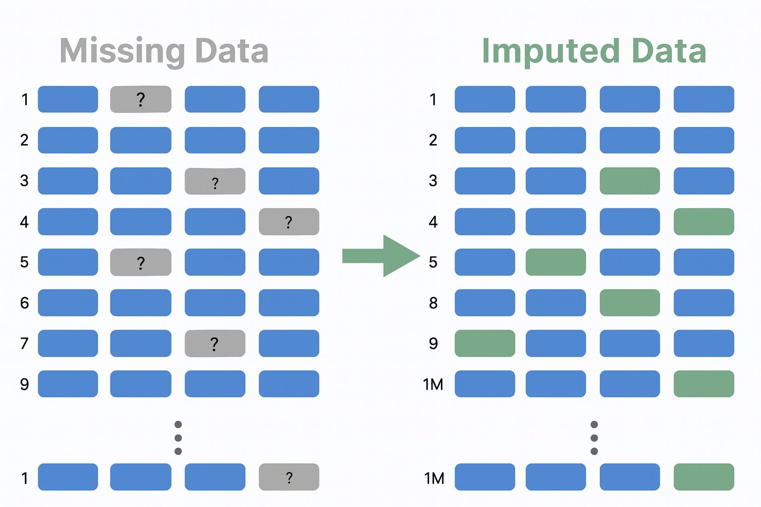
In observe, most real-world datasets comprise lacking values, making lacking information one of the crucial frequent challenges in statistical modeling. If it’s not dealt with correctly, it will possibly result in biased coefficient estimates, decreased statistical energy, and in the end incorrect conclusions (Van Buuren, 2018). In predictive modeling, ignoring lacking information by performing full case evaluation or by excluding predictor variables with lacking values can restrict the applicability of the mannequin and lead to biased or suboptimal efficiency.

The Three Lacking-Knowledge Mechanisms

To handle this situation, statisticians classify lacking information into three mechanisms that describe how and why values go lacking. MCAR (Lacking Utterly at Random) refers to instances the place the missingness happens totally at random and is unbiased of each noticed and unobserved variables. MAR (Lacking at Random) signifies that the likelihood of missingness is determined by the noticed variables however not on the lacking worth itself. MNAR (Lacking Not at Random) describes probably the most complicated case, wherein the likelihood of missingness is determined by the unobserved worth itself.

Classical Approaches and Their Limits to take care of lacking information

Underneath the MAR assumption, it’s doable to make use of the knowledge contained within the noticed variables to foretell the lacking values. Classical approaches primarily based on this concept embrace regression-based imputation, k-nearest neighbors (kNN) imputation, and a number of imputation by chained equations (MICE). These strategies are thought-about multivariate as a result of they explicitly situation the imputation on the noticed variables.These approaches explicitly situation the imputation on the noticed information, however have a big limitation: they don’t deal with blended databases (steady + categorical) effectively and have problem capturing nonlinear relationships and sophisticated interactions.

The Rise of MissForest applied in R

It’s to beat these limitations that MissForest (Stekhoven & Bühlmann, 2012) has established itself as a benchmark methodology. Primarily based on random forests, MissForest can seize nonlinear relationships and sophisticated interactions between variables, typically outperforming conventional imputation strategies. Nonetheless, when engaged on a undertaking that required a generalizable modeling course of — with a correct practice/check break up and out-of-time validation — we encountered a big limitation. The R implementation of the missForest package deal doesn’t retailer the imputation mannequin parameters as soon as fitted.

A Essential Limitation of MissForest in Prediction Settings

This creates a sensible problem: it’s not possible to coach the imputation mannequin on the coaching set after which apply the very same parameters to the check set. This limitation introduces a danger of data leakage throughout mannequin analysis or a degradation within the high quality and consistency of imputations.

Current options and Their Dangers

Whereas on the lookout for another resolution that might permit constant imputation in a predictive modeling setting, we requested ourselves a easy however important query:

How can we impute the check information in a manner that continues to be totally in step with the imputations realized on the coaching information?

Exploring this query led us to a dialogue on CrossValidated, the place one other consumer was dealing with the very same situation and requested:

“Learn how to use missForest in R for check information imputation?”

Two principal options had been urged to beat this limitation. The primary consists of merging the coaching and check information earlier than working the imputation. This strategy typically improves the standard of the imputations as a result of the algorithm has extra information to be taught from, however it introduces information leakage, for the reason that check set influences the imputation mannequin. The second strategy imputes the check set individually from the coaching set, which prevents data leakage however forces the algorithm to construct a completely new imputation mannequin utilizing solely the check information, which is usually a lot smaller. This will result in much less steady imputations and a possible drop in predictive efficiency.

Even the well-known tutorial by Liam Morgan arrives at an analogous workaround. His proposed resolution includes imputing the coaching set, becoming a predictive mannequin, then combining the coaching and check information for a last imputation step:

# 1) Impute the coaching set
imp_train_X <- missForest(train_X)$ximp

# 2) Construct the predictive mannequin
rf <- randomForest(x = imp_train_X, y = practice$creditability)

# 3) Mix practice and check, then re-impute
train_test_X <- rbind(test_X, imp_train_X)
imp_test_X <- missForest(train_test_X)$ximp[1:nrow(test_X), ]

Though this strategy typically could improves imputation high quality, it suffers from the identical weak spot as Methodology 1: the check information not directly take part within the studying course of, which can inflate mannequin efficiency metrics and creates an excessively optimistic estimate of generalization.

These examples spotlight a elementary dilemma:

• How will we impute lacking values with out biasing mannequin analysis?
• How will we be sure that the imputations utilized to the check set are in step with these realized on the coaching set?

Analysis Query and Motivation

These questions motivated our exploration of a extra sturdy resolution that preserves generalization, avoids information leakage, and produces steady imputations appropriate for predictive modeling pipelines.

This paper is organized into 4 principal sections:

• Part 1 introduces the method of figuring out and characterizing lacking values, together with the best way to detect, quantify, and describe them.
• Part 2 discusses the MCAR (Lacking Utterly at Random) mechanism and presents strategies for dealing with lacking information below this assumption.
• Part 3 focuses on the MAR (Lacking at Random) mechanism, outlining applicable imputation methods and addressing the important query: Why does the MissForest implementation in R fail in prediction settings?
• Part 4 examines the MNAR (Lacking Not at Random) mechanism and explores methods for coping with lacking information when the mechanism is determined by the unobserved values themselves.

1. Identification and Characterization of Lacking Values

This step is important and ought to be carried out in shut collaboration with all stakeholders: mannequin builders, area specialists, and future customers of the mannequin. The purpose is to establish all lacking values and mark them.

In Python, and notably when utilizing libraries comparable to Pandas, NumPy, and Scikit-Study, lacking values are represented as NaN. Values marked as NaN are ignored by many operations comparable to sum() and rely(). You’ll be able to mark lacking values utilizing the exchange() operate on the related subset of columns in a Pandas DataFrame.

As soon as the lacking values have been marked, the subsequent step is to judge their distribution for every variable. The isnull() operate can be utilized to establish all NaN values as True, and mixed with sum() to rely the variety of lacking values per column.

Understanding the distribution of lacking values is essential. With this data, stakeholders can assess whether or not the patterns of missingness are affordable. It additionally means that you can outline acceptable thresholds of missingness relying on the character of every variable. For example, you would possibly resolve that as much as 10% lacking values is suitable for steady variables, whereas the edge for categorical variables ought to stay at 0%.

After deciding on the related variables for modeling, together with these containing lacking values when they’re vital for prediction, it’s important to separate the dataset into three samples:

• Coaching set to estimate parameters and practice the fashions,
• Check set to judge mannequin efficiency on unseen information,
• Out-of-Time (OOT) set to validate the temporal robustness of the mannequin.

This break up ought to be carried out to protect the statistical representativeness of every subsample — for instance, through the use of stratified sampling if the goal variable is imbalanced.

The evaluation of lacking values ought to then be performed completely on the coaching set:

• Establish their mechanism (MCAR, MAR, MNAR) utilizing statistical checks,
• Choose the suitable imputation methodology,
• Practice the imputation fashions on the coaching set.

The imputation parameters and fashions obtained on this step should then be utilized as is to the check set and to the Out-of-Time set. This step is crucial to keep away from data leakage and to make sure an accurate analysis of the mannequin’s generalization efficiency.

Within the subsequent part, we are going to look at the MCAR mechanism intimately and current the imputation strategies which can be finest fitted to this sort of lacking information.

2. Understanding MCAR and Selecting the Proper Imputation Strategies

In easy phrases, MCAR (Lacking Utterly at Random) describes a scenario the place the truth that a worth is lacking is totally unrelated to both the worth itself or another variables within the dataset. In mathematical phrases, which means the likelihood of an information level being lacking doesn’t depend upon the variable’s worth nor on the values of another variables: the missingness is totally random.

Earlier than formally defining the MCAR mechanism, allow us to introduce the notations that will probably be used on this part and all through the article:

• Think about an unbiased and identically distributed pattern of n observations:

y_i = (y_i1, . . ., y_ip)^T, i = 1, 2, . . ., n

the place p is the variety of variables with lacking values and n is the pattern measurement.

• Y ∈ R^nxp represents the variables that will comprise lacking values. That is the set on which we want to carry out imputation.

• We denote the noticed entries and lacking entries of Y as Y_o and Y_m,

• X ∈ R^nxq represents the totally noticed variables, which means they comprise no lacking values.
• To point which parts of y_i are noticed or lacking, we outline the indicator vector:

r_i = (r_i1, . . ., r_ip)^T, i = 1, 2, . . ., n

with r_ik = 1 if y_ik is noticed, and 0 in any other case.

• Stacking these vectors yields the entire matrix of presence/absence indicators:

R = (r₁, . . ., r_n)^T

Then the MCAR assumption is outlined as :

Pr(R|Y_m ,Y_o, X) = Pr(R). (1)

which means that the lacking indicators are fully unbiased of each the lacking information, Ym, and the noticed information, Y_o. Observe that right here R can be unbiased of covariates X. Earlier than presenting strategies for dealing with lacking values below the MCAR assumption, we are going to first introduce a number of easy strategies to evaluate whether or not the MCAR assumption is more likely to maintain.

2.1 Assessing the MCAR Assumption

On this part, we are going to simulate a dataset with 10,000 observations and 4 variables below the MCAR assumption:

• One steady variable containing 20% lacking values and one categorical variable with two ranges (0 and 1) containing 10% lacking values.
• One steady variable and one categorical variable which can be totally noticed, with no lacking values.
• Lastly, a binary goal variable named goal, taking values 0 and 1.

import numpy as np
import pandas as pd

# --- Reproducibility ---
np.random.seed(42)

# --- Parameters ---
n = 10000

# --- Utility Capabilities ---
def generate_continuous(imply, std, measurement, missing_rate=0.0):
    """Generate a steady variable with optionally available MCAR missingness."""
    values = np.random.regular(loc=imply, scale=std, measurement=measurement)
    if missing_rate > 0:
        masks = np.random.rand(measurement) < missing_rate
        values[mask] = np.nan
    return values

def generate_categorical(ranges, probs, measurement, missing_rate=0.0):
    """Generate a categorical variable with optionally available MCAR missingness."""
    values = np.random.selection(ranges, measurement=measurement, p=probs).astype(float)
    if missing_rate > 0:
        masks = np.random.rand(measurement) < missing_rate
        values[mask] = np.nan
    return values

# --- Variable Technology ---
variables = {
    "cont_mcar": generate_continuous(imply=100, std=20, measurement=n, missing_rate=0.20),
    "cat_mcar": generate_categorical(ranges=[0, 1], probs=[0.7, 0.3], measurement=n, missing_rate=0.10),
    "cont_full": generate_continuous(imply=50, std=10, measurement=n),
    "cat_full": generate_categorical(ranges=[0, 1], probs=[0.6, 0.4], measurement=n),
    "goal": np.random.selection([0, 1], measurement=n, p=[0.5, 0.5])
}

# --- Construct DataFrame ---
df = pd.DataFrame(variables)

# --- Show Abstract ---
print(df.head())
print("nMissing worth counts:")
print(df.isnull().sum())

Earlier than performing any evaluation, it’s important to separate the dataset into two components: a coaching set and a check set.

2.1.1 Making ready Practice and Check Knowledge for Evaluation the MCAR

It’s important to separate the dataset into coaching and check units whereas making certain representativeness. This ensures that each the mannequin and the imputation strategies are realized completely on the coaching set after which evaluated on the check set. Doing so prevents information leakage and offers an unbiased estimate of the mannequin’s means to generalize to unseen information.

from sklearn.model_selection import train_test_split
import pandas as pd

def stratified_split(df, strat_vars, test_size=0.3, random_state=None):
    """
    Break up a DataFrame into practice and check units with stratification
    primarily based on one or a number of variables.

    Parameters
    ----------
    df : pandas.DataFrame
        The enter dataset.
    strat_vars : checklist or str
        Column title(s) used for stratification.
    test_size : float, default=0.3
        Proportion of the dataset to incorporate within the check break up.
    random_state : int, optionally available
        Random seed for reproducibility.

    Returns
    -------
    train_df : pandas.DataFrame
        Coaching set.
    test_df : pandas.DataFrame
        Check set.
    """
    # Guarantee strat_vars is an inventory
    if isinstance(strat_vars, str):
        strat_vars = [strat_vars]

    # Create a mixed stratification key
    strat_key = df[strat_vars].astype(str).fillna("MISSING").agg("_".be part of, axis=1)

    # Carry out stratified break up
    train_df, test_df = train_test_split(
        df,
        test_size=test_size,
        stratify=strat_key,
        random_state=random_state
    )

    return train_df, test_df


# --- Software ---
# Stratification sur cat_mcar, cat_full et goal
train_df, test_df = stratified_split(df, strat_vars=["cat_mcar", "cat_full", "target"], test_size=0.3, random_state=42)

print(f"Practice measurement: {train_df.form[0]}  ({len(train_df)/len(df):.1%})")
print(f"Check measurement:  {test_df.form[0]}  ({len(test_df)/len(df):.1%})")

2.1.1 Evaluation MCAR Assumption for steady variables with lacking values

Step one is to create a binary indicator R (the place 1 signifies an noticed worth and 0 signifies a lacking worth) and evaluate the distributions of Yo​, Ym​, and X throughout the 2 teams (noticed vs. lacking).

Allow us to illustrate this course of utilizing the variable cont_mcar for example. We are going to evaluate the distribution of cont_full between observations the place cont_mcar is lacking and the place it’s noticed, utilizing each a boxplot and a Kolmogorov–Smirnov check. We are going to then carry out an analogous evaluation for the specific variable cat_full, evaluating proportions throughout the 2 teams with a bar plot and a chi-squared check.

import matplotlib.pyplot as plt
import seaborn as sns

# --- Step 1: Practice/Check Break up with Stratification ---
train_df, test_df = stratified_split(
    df,
    strat_vars=["cat_mcar", "cat_full", "target"],
    test_size=0.3,
    random_state=42
)

# --- Step 2: Create the R indicator on the coaching set ---
train_df = train_df.copy()
train_df["R_cont_mcar"] = np.the place(train_df["cont_mcar"].isnull(), 0, 1)

# --- Step 3: Put together the information for comparability ---
df_obs = pd.DataFrame({
    "cont_full": train_df.loc[train_df["R_cont_mcar"] == 1, "cont_full"],
    "Group": "Noticed (R=1)"
})

df_miss = pd.DataFrame({
    "cont_full": train_df.loc[train_df["R_cont_mcar"] == 0, "cont_full"],
    "Group": "Lacking (R=0)"
})

df_all = pd.concat([df_obs, df_miss])

# --- Step 4: KS Check earlier than plotting ---
from scipy.stats import ks_2samp
stat, p_value = ks_2samp(
    train_df.loc[train_df["R_cont_mcar"] == 1, "cont_full"],
    train_df.loc[train_df["R_cont_mcar"] == 0, "cont_full"]
)

# --- Step 5: Visualization with KS end result ---
plt.determine(figsize=(8, 6))
sns.boxplot(
    x="Group", 
    y="cont_full", 
    information=df_all,
    palette="Set2",
    width=0.6,
    fliersize=3
)

# Add crimson diamonds for means
means = df_all.groupby("Group")["cont_full"].imply()
for i, m in enumerate(means):
    plt.scatter(i, m, shade="crimson", marker="D", s=50, zorder=3, label="Imply" if i == 0 else "")

# Title and KS check end result
plt.title("Distribution of cont_full by Missingness of cont_mcar (Practice Set)",
          fontsize=14, weight="daring")

# Add KS end result as textual content field
textstr = f"KS Statistic = {stat:.3f}nP-value = {p_value:.3f}"
plt.gca().textual content(
    0.05, 0.95, textstr,
    rework=plt.gca().transAxes,
    fontsize=10,
    verticalalignment='high',
    bbox=dict(boxstyle="spherical,pad=0.3", facecolor="white", alpha=0.8)
)

plt.ylabel("cont_full", fontsize=12)
plt.xlabel("")
sns.despine()
plt.legend()
plt.present()

import seaborn as sns
import matplotlib.pyplot as plt
from scipy.stats import chi2_contingency

# --- Step 1: Construct contingency desk on the TRAIN set ---
contingency_table = pd.crosstab(train_df["R_cont_mcar"], train_df["cat_full"])
chi2, p_value, dof, anticipated = chi2_contingency(contingency_table)

# --- Step 2: Compute proportions for every group ---
# --- Recompute proportions however flip the axes ---
props = contingency_table.div(contingency_table.sum(axis=1), axis=0)

# Rework for plotting: Group (R) on x-axis, Class as hue
df_props = props.reset_index().soften(
    id_vars="R_cont_mcar",
    var_name="Class",
    value_name="Proportion"
)

# Map R values to clear labels
df_props["Group"] = df_props["R_cont_mcar"].map({1: "Noticed (R=1)", 0: "Lacking (R=0)"})

# --- Plot: Group on x-axis, bars present proportions of every class ---
sns.set_theme(model="whitegrid")
plt.determine(figsize=(8,6))

sns.barplot(
    x="Group", y="Proportion", hue="Class",
    information=df_props, palette="Set2"
)

# Title and Chi² end result
plt.title("Proportion of cat_full by Noticed/Lacking Standing of cont_mcar (Practice Set)",
          fontsize=14, weight="daring")

# Add Chi² end result as a textual content field
textstr = f"Chi² = {chi2:.3f}, p = {p_value:.3f}"
plt.gca().textual content(
    0.05, 0.95, textstr,
    rework=plt.gca().transAxes,
    fontsize=10,
    verticalalignment='high',
    bbox=dict(boxstyle="spherical,pad=0.3", facecolor="white", alpha=0.8)
)

plt.xlabel("Noticed / Lacking Group (R)")
plt.ylabel("Proportion")
plt.legend(title="cat_full Class")
sns.despine()
plt.present()

The 2 figures above present that, below the MCAR assumption, the distribution of 𝑌​, 𝑌ₘ​, and 𝑋 stays unchanged whatever the worth of R (1 = noticed, 0 = lacking). These outcomes are additional supported by the Kolmogorov–Smirnov and Chi-squared checks, which affirm the absence of serious variations between the noticed and lacking teams.

For categorical variables, the identical analyses might be carried out as described above. Whereas these univariate checks might be time-consuming, they’re helpful when the variety of variables is small, as they supply a fast and intuitive first have a look at the lacking information mechanism. For bigger datasets, nevertheless, multivariate strategies ought to be thought-about.

2.1.3 Multivariate Evaluation of the MCAR Assumption

To the perfect of my information, just one multivariate statistical check is extensively used to evaluate the MCAR assumption on the dataset degree: Little’s chi2 for check MCAR assumption referred to as mcartest. This check, developed in R language, compares the distributions of noticed variables throughout totally different missing-data patterns and computes a worldwide check statistic that follows a Chi-squared distribution.

Nonetheless, its principal limitation is that it’s not effectively fitted to categorical variables, because it depends on the robust assumption that the variables are usually distributed. We now flip to the strategies for imputing lacking values below the MCAR assumption.

2.2 Strategies to take care of lacking information below MCAR.

Underneath the MCAR assumption, the missingness indicators R are unbiased of Y_o, Y_m, and X. Because the information are lacking fully at random, dropping incomplete observations doesn’t introduce bias. Nonetheless, this strategy turns into inefficient when the proportion of lacking values is excessive.

In such instances, easy imputation strategies, changing lacking values with the imply, median, or most frequent class, are sometimes most popular. They’re straightforward to implement, require little computational effort, and might be managed over time with out including complexity for modelers. Whereas these strategies don’t create bias, they have a tendency to underestimate variance and should distort relationships between variables.

Against this, superior strategies comparable to regression-based imputation, kNN, or a number of imputation can enhance statistical effectivity and assist protect data when the proportion of lacking information is substantial. Their principal downside lies of their algorithmic complexity, larger computational price, and the better effort required to take care of them in manufacturing settings.

To impute lacking values below the MCAR assumption for prediction functions, proceed as follows:

1. Study imputation values from the coaching set solely, utilizing the imply for steady variables and probably the most frequent class for categorical variables.
2. Apply these values to interchange lacking information in each the coaching and the check units.
3. Consider the mannequin on the check set, making certain that no data from the check set was used through the imputation course of.

import pandas as pd

def compute_impute_values(df, cont_vars, cat_vars):
    """
    Compute imputation values (imply for steady, mode for categorical)
    from the coaching set solely.
    """
    impute_values = {}
    for col in cont_vars:
        impute_values[col] = df[col].imply()
    for col in cat_vars:
        impute_values[col] = df[col].mode().iloc[0]
    return impute_values

def apply_imputation(train_df, test_df, impute_values, vars_to_impute):
    """
    Apply the realized imputation values to each practice and check units.
    """
    train_df[vars_to_impute] = train_df[vars_to_impute].fillna(worth=impute_values)
    test_df[vars_to_impute] = test_df[vars_to_impute].fillna(worth=impute_values)
    return train_df, test_df

# --- Instance utilization ---
train_df, test_df = stratified_split(
    df,
    strat_vars=["cat_mcar", "cat_full", "target"],
    test_size=0.3,
    random_state=42
)

# Variables to impute
cont_vars = ["cont_mcar"]
cat_vars = ["cat_mcar"]
vars_to_impute = cont_vars + cat_vars

# 1. Study imputation values on TRAIN
impute_values = compute_impute_values(train_df, cont_vars, cat_vars)
print("Imputation values realized from practice:", impute_values)

# 2. Apply them constantly to TRAIN and TEST
train_df, test_df = apply_imputation(train_df, test_df, impute_values, vars_to_impute)

# 3. Verify
print("Remaining lacking values in practice:n", train_df[vars_to_impute].isnull().sum())
print("Remaining lacking values in check:n", test_df[vars_to_impute].isnull().sum())

This part on understanding MCAR and deciding on the suitable imputation methodology offers a transparent basis for approaching comparable methods below the MAR assumption.

3. Understanding MAR and Selecting the Proper Imputation Strategies

The MAR assumption is outlined as :

Pr(R|Y_m ,Y_o, X) = Pr(R|Y_o, X) (2)

In different phrases, the distribution of the lacking indicators relies upon solely on the noticed information. Even within the case the place R relies upon solely on the covariates X,

Pr(R|Y_m ,Y_o, X) = Pr(R|X) (3)

This nonetheless falls below the MAR assumption.

3.1 Evaluation MAR Assumption for variables with lacking values

Underneath the MAR assumption, the missingness indicators 𝑅 rely solely on the noticed variables Y_o and X, however not on the lacking information 𝑌.
To not directly assess the plausibility of this assumption, frequent statistical checks (Scholar’s t-test, Kolmogorov–Smirnov, Chi-squared, and many others.) might be utilized by evaluating the distributions of noticed variables between teams with and with out lacking values.

For multivariate evaluation, one may use the mcartest applied in R, which extends Little’s check of MCAR to judge assumption (3), particularly Pr(R|Y_m ,Y_o, X) = Pr(R|X), below the idea of multivariate normality of the variables.

If this check isn’t rejected, the missing-data mechanism can fairly be thought-about MAR (assumption 3) given the auxiliary variables X .

We are able to now flip to the query of the best way to impute this sort of lacking information.

3.2 Strategies to take care of lacking information below MAR.

Underneath the MAR assumption, the likelihood of missingness R relies upon solely on the noticed variables Y_o​ and covariates X. On this setting, variables Y^ok with lacking values might be defined utilizing the opposite obtainable variables Y_o and X, which motivates the usage of superior imputation strategies primarily based on supervised studying.

These approaches contain constructing a predictive mannequin wherein the unfinished variable Y^ok serves because the goal, and the opposite noticed variables Y_o and X act as predictors. The mannequin is skilled on full instances ([Y^k]_o of Y) after which utilized to estimate the lacking values [Y^k​]_m of Y^ok.

Essentially the most generally used imputation strategies within the literature embrace:

• k-nearest neighbors (KNNimpute, Troyanskaya et al., 2001), primarily utilized to steady information;
• the saturated multinomial mannequin (Schafer, 1997), designed for categorical information;
• multivariate imputation by chained equations (MICE, Van Buuren & Oudshoorn, 1999), appropriate for blended datasets however depending on tuning parameters and the specification of a parametric mannequin.

All of those approaches depend on assumptions concerning the underlying information distribution or on the power of the chosen mannequin to adequately seize relationships between variables.

Extra just lately, MissForest (Stekhoven & Bühlmann, 2012) has emerged as a nonparametric different primarily based on random forests, well-suited to blended information sorts and sturdy to each interactions and nonlinear relationships.

The MissForest algorithm depends on random forests (RF) to impute lacking values. The authors suggest the next process:

As outlined, the MissForest algorithm can’t be used straight for prediction functions. For every variable, between steps 6 and seven, the random forest mannequin M_s​ used to foretell y_mis(s)​ from x_mis(s)​isn’t saved. Consequently, it’s neither doubtless nor fascinating for practitioners to depend on MissForest as a predictive mannequin in manufacturing.

The absence of saved fashions M_s​ or imputation parameters (right here on the coaching set) makes it tough to judge generalization efficiency on new information. Though some have tried to work round this situation by following Liam Morgan‘s strategy, the problem stays unresolved.

Moreover, this limitation will increase algorithmic complexity and computational price, for the reason that total algorithm have to be rerun from scratch for every new dataset (as an example, when working with separate coaching and check units).

What ought to be carried out? Ought to the MissForest algorithm nonetheless be used?

If the purpose is to develop a mannequin for classification or evaluation solely on the obtainable dataset, with no intention of making use of it to new information, then MissForest is strongly advisable, because it gives excessive accuracy and robustness.

Nonetheless, if the purpose is to construct a predictive mannequin that will probably be utilized to new datasets, MissForest ought to be prevented for the explanations mentioned above. In such instances, it’s preferable to make use of an algorithm that explicitly shops the imputation fashions or the parameters estimated from the coaching set.

Thankfully, an tailored model now exists: MissForestPredict, obtainable since 2024 in each R and Python, particularly designed for predictive duties. For additional particulars, we refer the reader to Albu, Elena, et al. (2024).

Using the MissForestPredict algorithm for prediction consists of making use of the usual MissForest process to the coaching information. In contrast to the unique MissForest, nevertheless, this model returns and shops the person fashions M_s related to every variable, which makes it doable to reuse them for imputing lacking values in new datasets.

The algorithm under illustrates the best way to apply MissForestPredict to new observations, whether or not they come from the check set, an out-of-time pattern, or an software dataset.

We now have all the weather wanted to handle the problems raised within the introduction. Allow us to flip to the ultimate mechanism, MNAR, earlier than transferring on to the conclusion.

4. Understanding MNAR

Lacking Not At Random (MNAR) happens when the lacking information mechanism relies upon straight on the unobserved values themselves. In different phrases, if a variable Y comprises lacking values, then the indicator variable R (with R=1 if Y is noticed and R=0 in any other case) relies upon solely on the lacking element Y_m.

There isn’t any common statistical methodology to deal with this sort of mechanism, for the reason that data wanted to mannequin the dependency is exactly what’s lacking. In such instances, the advisable strategy is to depend on area experience to grasp the explanations behind the nonresponse and to outline context-specific methods for analyzing and addressing the lacking values.

You will need to emphasize, nevertheless, that MAR and MNAR can’t usually be distinguished empirically primarily based on the noticed information alone.

Conclusion

The target of this text was to indicate the best way to impute lacking values for predictive functions with out biasing the analysis of mannequin efficiency. To this finish, we introduced the principle mechanisms that generate lacking information (MCAR, MAR, MNAR), the statistical checks used to evaluate their plausibility, and the imputation strategies finest suited to every.

Our evaluation highlights that, below MCAR, easy imputation strategies are usually preferable, as they supply substantial time financial savings with out introducing bias. In observe, nevertheless, lacking information mechanisms are most frequently MAR. On this setting, superior imputation approaches comparable to MissForest, primarily based on machine studying fashions, are notably applicable.

Nonetheless, when the purpose is to construct predictive fashions, it’s important to make use of strategies that retailer the imputation parameters or fashions realized from the coaching information after which replicate them constantly on the check, out-of-time, or software datasets. That is exactly the contribution of MissForestPredict (launched in 2024 and obtainable in each R and Python), which addresses the limitation of the unique MissForest (2012), a technique not initially designed for predictive duties.

Utilizing MissForest for prediction with out adaptation could subsequently result in biased outcomes, until corrective measures are applied. It could be extremely helpful for practitioners who’ve deployed MissForest in manufacturing to share the methods they developed to beat this limitation.

References

[1] Audigier, V., White, I. R., Jolani, S., Debray, T. P., Quartagno, M., Carpenter, J., … & Resche-Rigon, M. (2018). A number of imputation for multilevel information with steady and binary variables.

[2] Stekhoven, D. J., & Bühlmann, P. (2012). MissForest—non-parametric lacking worth imputation for mixed-type information. Bioinformatics, 28(1), 112-118.

[3] Li, C. (2013). Little’s check of lacking fully at random. The Stata Journal, 13(4), 795-809.

[4] Albu, E., Gao, S., Wynants, L., & Van Calster, B. (2024). missForestPredict–Lacking information imputation for prediction settings. arXiv preprint arXiv:2407.03379.

Picture Credit

All pictures and visualizations on this article had been created by the writer utilizing Python (pandas, matplotlib, seaborn, and plotly) and excel, until in any other case acknowledged.

Disclaimer

I write to be taught so errors are the norm, despite the fact that I strive my finest. Please, while you spot them, let me know. I additionally respect strategies on new matters!