


On this article, you’ll learn to fuse dense LLM sentence embeddings, sparse TF-IDF options, and structured metadata right into a single scikit-learn pipeline for textual content classification.
Matters we are going to cowl embody:
- Loading and making ready a textual content dataset alongside artificial metadata options.
- Constructing parallel function pipelines for TF-IDF, LLM embeddings, and numeric metadata.
- Fusing all function branches with
ColumnTransformerand coaching an end-to-end classifier.
Let’s break it down.

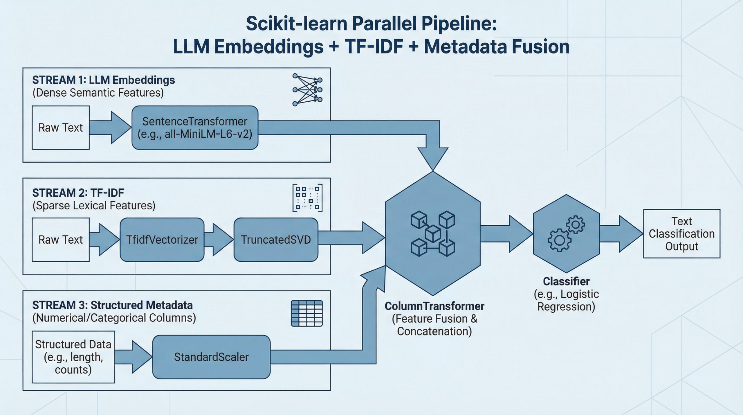
The way to Mix LLM Embeddings + TF-IDF + Metadata in One Scikit-learn Pipeline (click on to enlarge)
Picture by Editor
Introduction
Knowledge fusion, or combining various items of knowledge right into a single pipeline, sounds bold sufficient. If we discuss not nearly two, however about three complementary function sources, then the problem — and the potential payoff — goes to the subsequent stage. Essentially the most thrilling half is that scikit-learn permits us to unify all of them cleanly inside a single, end-to-end workflow. Do you need to see how? This text walks you step-by-step by constructing an entire fusion pipeline from scratch for a downstream textual content classification activity, combining dense semantic info from LLM-generated embeddings, sparse lexical options from TF-IDF, and structured metadata indicators. ? Hold studying.
Step-by-Step Pipeline Constructing Course of
First, we are going to make all the required imports for the pipeline-building course of. If you’re working in a neighborhood surroundings, you would possibly must pip set up a few of them first:
|
import numpy as np import pandas as pd
from sklearn.datasets import fetch_20newsgroups from sklearn.model_selection import train_test_split from sklearn.pipeline import Pipeline from sklearn.compose import ColumnTransformer from sklearn.feature_extraction.textual content import TfidfVectorizer from sklearn.preprocessing import StandardScaler from sklearn.linear_model import LogisticRegression from sklearn.metrics import classification_report from sklearn.base import BaseEstimator, TransformerMixin from sklearn.decomposition import TruncatedSVD
from sentence_transformers import SentenceTransformer |
Let’s look intently at this — virtually countless! — listing of imports. I wager one factor has caught your consideration: fetch_20newsgroups. It is a freely obtainable textual content dataset in scikit-learn that we are going to use all through this text: it incorporates textual content extracted from information articles belonging to all kinds of classes.
To maintain our dataset manageable in apply, we are going to decide the information articles belonging to a subset of classes specified by us. The next code does the trick:
|
1 2 3 4 5 6 7 8 9 10 11 12 13 14 15 16 17 |
classes = [ “rec.sport.baseball”, “sci.space”, “comp.graphics”, “talk.politics.misc” ]
dataset = fetch_20newsgroups( subset=“all”, classes=classes, take away=(“headers”, “footers”, “quotes”) )
X_raw = dataset.knowledge y = dataset.goal
print(f“Variety of samples: {len(X_raw)}”) |
We known as this freshly created dataset X_raw to emphasise that it is a uncooked, far-from-final model of the dataset we are going to progressively assemble for downstream duties like utilizing machine studying fashions for predictive functions. It’s truthful to say that the “uncooked” suffix can be used as a result of right here now we have the uncooked textual content, from which three totally different knowledge elements (or streams) will likely be generated and later merged.
For the structured metadata related to the information articles obtained, in real-world contexts, this metadata would possibly already be obtainable or supplied by the dataset proprietor. That’s not the case with this publicly obtainable dataset, so we are going to synthetically create some easy metadata options primarily based on the textual content, together with options describing character size, phrase depend, common phrase size, uppercase ratio, and digit ratio.
|
1 2 3 4 5 6 7 8 9 10 11 12 13 14 15 16 17 18 19 20 21 22 23 24 25 26 27 28 29 30 31 32 33 34 35 36 37 38 39 |
def generate_metadata(texts): lengths = [len(t) for t in texts] word_counts = [len(t.split()) for t in texts]
avg_word_lengths = [] uppercase_ratios = [] digit_ratios = []
for t in texts: phrases = t.break up() if phrases: avg_word_lengths.append(np.imply([len(w) for w in words])) else: avg_word_lengths.append(0)
denom = max(len(t), 1)
uppercase_ratios.append( sum(1 for c in t if c.isupper()) / denom )
digit_ratios.append( sum(1 for c in t if c.isdigit()) / denom )
return pd.DataFrame({ “textual content”: texts, “char_length”: lengths, “word_count”: word_counts, “avg_word_length”: avg_word_lengths, “uppercase_ratio”: uppercase_ratios, “digit_ratio”: digit_ratios })
# Calling the operate to generate a structured dataset that incorporates: uncooked textual content + metadata df = generate_metadata(X_raw) df[“target”] = y
df.head() |
Earlier than getting absolutely into the pipeline-building course of, we are going to break up the info into prepare and check subsets:
|
X = df.drop(columns=[“target”]) y = df[“target”]
X_train, X_test, y_train, y_test = train_test_split( X, y, test_size=0.2, random_state=42, stratify=y ) |
Essential: splitting the info into coaching and check units should be executed earlier than extracting the LLM embeddings and TF-IDF options. Why? As a result of these two extraction processes develop into a part of the pipeline, they usually contain becoming transformations with scikit-learn, that are studying processes — for instance, studying the TF-IDF vocabulary and inverse doc frequency (IDF) statistics. The scikit-learn logic to implement that is as follows: any knowledge transformations should be fitted (study the transformation logic) solely on the coaching knowledge after which utilized to the check knowledge utilizing the realized logic. This fashion, no info from the check set will affect or bias function building or downstream mannequin coaching.
Now comes a key stage: defining a category that encapsulates a pre-trained sentence transformer (a language mannequin like all-MiniLM-L6-v2 able to producing textual content embeddings from uncooked textual content) to provide our customized LLM embeddings.
|
class EmbeddingTransformer(BaseEstimator, TransformerMixin): def __init__(self, model_name=“all-MiniLM-L6-v2”): self.model_name = model_name self.mannequin = None
def match(self, X, y=None): self.mannequin = SentenceTransformer(self.model_name) return self
def remodel(self, X): embeddings = self.mannequin.encode( X.tolist(), show_progress_bar=False ) return np.array(embeddings) |
Now we’re constructing the three principal knowledge branches (or parallel pipelines) we’re interested by, one after the other. First, the pipeline for TF-IDF function extraction, wherein we are going to use scikit-learn’s TfidfVectorizer class to extract these options seamlessly:
|
tfidf_pipeline = Pipeline([ (“tfidf”, TfidfVectorizer(max_features=5000)), (“svd”, TruncatedSVD(n_components=300, random_state=42)) ]) |
Subsequent comes the LLM embeddings pipeline, aided by the customized class we outlined earlier:
|
embedding_pipeline = Pipeline([ (“embed”, EmbeddingTransformer()) ]) |
Final, we outline the department pipeline for the metadata options, wherein we purpose to standardize these attributes because of their disparate ranges:
|
metadata_features = [ “char_length”, “word_count”, “avg_word_length”, “uppercase_ratio”, “digit_ratio” ]
metadata_pipeline = Pipeline([ (“scaler”, StandardScaler()) ]) |
Now now we have three parallel pipelines, however nothing to attach them — at the least not but. Right here comes the principle, overarching pipeline that may orchestrate the fusion course of amongst all three knowledge branches, through the use of a really helpful and versatile scikit-learn artifact for the fusion of heterogeneous knowledge flows: a ColumnTransformer pipeline.
|
preprocessor = ColumnTransformer( transformers=[ (“tfidf”, tfidf_pipeline, “text”), (“embedding”, embedding_pipeline, “text”), (“metadata”, metadata_pipeline, metadata_features), ], the rest=“drop” ) |
And the icing on the cake: a full, end-to-end pipeline that may mix the fusion pipeline with an instance of a machine learning-driven downstream activity. Specifically, right here’s the best way to mix the complete knowledge fusion pipeline now we have simply architected with the coaching of a logistic regression classifier to foretell the information class:
|
full_pipeline = Pipeline([ (“features”, preprocessor), (“clf”, LogisticRegression(max_iter=2000)) ]) |
The next instruction will do all of the heavy lifting now we have been designing to date. The LLM embeddings half will significantly take a couple of minutes (particularly if the mannequin must be downloaded), so be affected person. This step will undertake the entire threefold course of of knowledge preprocessing, fusion, and mannequin coaching:
|
full_pipeline.match(X_train, y_train) |
To finalize, we are able to make predictions on the check set and see how our fusion-driven classifier performs.
|
y_pred = full_pipeline.predict(X_test)
print(classification_report(y_test, y_pred, target_names=dataset.target_names)) |
And for a visible wrap-up, right here’s what the complete pipeline appears like:

Wrapping Up
This text guided you thru the method of constructing a whole machine learning-oriented workflow that focuses on the fusion of a number of info sources derived from uncooked textual content knowledge, in order that all the things may be put collectively in downstream predictive duties like textual content classification. Now we have seen how scikit-learn supplies a set of helpful lessons and strategies to make the method simpler and extra intuitive.
On this article, you’ll learn to fuse dense LLM sentence embeddings, sparse TF-IDF options, and structured metadata right into a single scikit-learn pipeline for textual content classification.
Matters we are going to cowl embody:
- Loading and making ready a textual content dataset alongside artificial metadata options.
- Constructing parallel function pipelines for TF-IDF, LLM embeddings, and numeric metadata.
- Fusing all function branches with
ColumnTransformerand coaching an end-to-end classifier.
Let’s break it down.
The way to Mix LLM Embeddings + TF-IDF + Metadata in One Scikit-learn Pipeline (click on to enlarge)
Picture by Editor
Introduction
Knowledge fusion, or combining various items of knowledge right into a single pipeline, sounds bold sufficient. If we discuss not nearly two, however about three complementary function sources, then the problem — and the potential payoff — goes to the subsequent stage. Essentially the most thrilling half is that scikit-learn permits us to unify all of them cleanly inside a single, end-to-end workflow. Do you need to see how? This text walks you step-by-step by constructing an entire fusion pipeline from scratch for a downstream textual content classification activity, combining dense semantic info from LLM-generated embeddings, sparse lexical options from TF-IDF, and structured metadata indicators. ? Hold studying.
Step-by-Step Pipeline Constructing Course of
First, we are going to make all the required imports for the pipeline-building course of. If you’re working in a neighborhood surroundings, you would possibly must pip set up a few of them first:
|
import numpy as np import pandas as pd
from sklearn.datasets import fetch_20newsgroups from sklearn.model_selection import train_test_split from sklearn.pipeline import Pipeline from sklearn.compose import ColumnTransformer from sklearn.feature_extraction.textual content import TfidfVectorizer from sklearn.preprocessing import StandardScaler from sklearn.linear_model import LogisticRegression from sklearn.metrics import classification_report from sklearn.base import BaseEstimator, TransformerMixin from sklearn.decomposition import TruncatedSVD
from sentence_transformers import SentenceTransformer |
Let’s look intently at this — virtually countless! — listing of imports. I wager one factor has caught your consideration: fetch_20newsgroups. It is a freely obtainable textual content dataset in scikit-learn that we are going to use all through this text: it incorporates textual content extracted from information articles belonging to all kinds of classes.
To maintain our dataset manageable in apply, we are going to decide the information articles belonging to a subset of classes specified by us. The next code does the trick:
|
1 2 3 4 5 6 7 8 9 10 11 12 13 14 15 16 17 |
classes = [ “rec.sport.baseball”, “sci.space”, “comp.graphics”, “talk.politics.misc” ]
dataset = fetch_20newsgroups( subset=“all”, classes=classes, take away=(“headers”, “footers”, “quotes”) )
X_raw = dataset.knowledge y = dataset.goal
print(f“Variety of samples: {len(X_raw)}”) |
We known as this freshly created dataset X_raw to emphasise that it is a uncooked, far-from-final model of the dataset we are going to progressively assemble for downstream duties like utilizing machine studying fashions for predictive functions. It’s truthful to say that the “uncooked” suffix can be used as a result of right here now we have the uncooked textual content, from which three totally different knowledge elements (or streams) will likely be generated and later merged.
For the structured metadata related to the information articles obtained, in real-world contexts, this metadata would possibly already be obtainable or supplied by the dataset proprietor. That’s not the case with this publicly obtainable dataset, so we are going to synthetically create some easy metadata options primarily based on the textual content, together with options describing character size, phrase depend, common phrase size, uppercase ratio, and digit ratio.
|
1 2 3 4 5 6 7 8 9 10 11 12 13 14 15 16 17 18 19 20 21 22 23 24 25 26 27 28 29 30 31 32 33 34 35 36 37 38 39 |
def generate_metadata(texts): lengths = [len(t) for t in texts] word_counts = [len(t.split()) for t in texts]
avg_word_lengths = [] uppercase_ratios = [] digit_ratios = []
for t in texts: phrases = t.break up() if phrases: avg_word_lengths.append(np.imply([len(w) for w in words])) else: avg_word_lengths.append(0)
denom = max(len(t), 1)
uppercase_ratios.append( sum(1 for c in t if c.isupper()) / denom )
digit_ratios.append( sum(1 for c in t if c.isdigit()) / denom )
return pd.DataFrame({ “textual content”: texts, “char_length”: lengths, “word_count”: word_counts, “avg_word_length”: avg_word_lengths, “uppercase_ratio”: uppercase_ratios, “digit_ratio”: digit_ratios })
# Calling the operate to generate a structured dataset that incorporates: uncooked textual content + metadata df = generate_metadata(X_raw) df[“target”] = y
df.head() |
Earlier than getting absolutely into the pipeline-building course of, we are going to break up the info into prepare and check subsets:
|
X = df.drop(columns=[“target”]) y = df[“target”]
X_train, X_test, y_train, y_test = train_test_split( X, y, test_size=0.2, random_state=42, stratify=y ) |
Essential: splitting the info into coaching and check units should be executed earlier than extracting the LLM embeddings and TF-IDF options. Why? As a result of these two extraction processes develop into a part of the pipeline, they usually contain becoming transformations with scikit-learn, that are studying processes — for instance, studying the TF-IDF vocabulary and inverse doc frequency (IDF) statistics. The scikit-learn logic to implement that is as follows: any knowledge transformations should be fitted (study the transformation logic) solely on the coaching knowledge after which utilized to the check knowledge utilizing the realized logic. This fashion, no info from the check set will affect or bias function building or downstream mannequin coaching.
Now comes a key stage: defining a category that encapsulates a pre-trained sentence transformer (a language mannequin like all-MiniLM-L6-v2 able to producing textual content embeddings from uncooked textual content) to provide our customized LLM embeddings.
|
class EmbeddingTransformer(BaseEstimator, TransformerMixin): def __init__(self, model_name=“all-MiniLM-L6-v2”): self.model_name = model_name self.mannequin = None
def match(self, X, y=None): self.mannequin = SentenceTransformer(self.model_name) return self
def remodel(self, X): embeddings = self.mannequin.encode( X.tolist(), show_progress_bar=False ) return np.array(embeddings) |
Now we’re constructing the three principal knowledge branches (or parallel pipelines) we’re interested by, one after the other. First, the pipeline for TF-IDF function extraction, wherein we are going to use scikit-learn’s TfidfVectorizer class to extract these options seamlessly:
|
tfidf_pipeline = Pipeline([ (“tfidf”, TfidfVectorizer(max_features=5000)), (“svd”, TruncatedSVD(n_components=300, random_state=42)) ]) |
Subsequent comes the LLM embeddings pipeline, aided by the customized class we outlined earlier:
|
embedding_pipeline = Pipeline([ (“embed”, EmbeddingTransformer()) ]) |
Final, we outline the department pipeline for the metadata options, wherein we purpose to standardize these attributes because of their disparate ranges:
|
metadata_features = [ “char_length”, “word_count”, “avg_word_length”, “uppercase_ratio”, “digit_ratio” ]
metadata_pipeline = Pipeline([ (“scaler”, StandardScaler()) ]) |
Now now we have three parallel pipelines, however nothing to attach them — at the least not but. Right here comes the principle, overarching pipeline that may orchestrate the fusion course of amongst all three knowledge branches, through the use of a really helpful and versatile scikit-learn artifact for the fusion of heterogeneous knowledge flows: a ColumnTransformer pipeline.
|
preprocessor = ColumnTransformer( transformers=[ (“tfidf”, tfidf_pipeline, “text”), (“embedding”, embedding_pipeline, “text”), (“metadata”, metadata_pipeline, metadata_features), ], the rest=“drop” ) |
And the icing on the cake: a full, end-to-end pipeline that may mix the fusion pipeline with an instance of a machine learning-driven downstream activity. Specifically, right here’s the best way to mix the complete knowledge fusion pipeline now we have simply architected with the coaching of a logistic regression classifier to foretell the information class:
|
full_pipeline = Pipeline([ (“features”, preprocessor), (“clf”, LogisticRegression(max_iter=2000)) ]) |
The next instruction will do all of the heavy lifting now we have been designing to date. The LLM embeddings half will significantly take a couple of minutes (particularly if the mannequin must be downloaded), so be affected person. This step will undertake the entire threefold course of of knowledge preprocessing, fusion, and mannequin coaching:
|
full_pipeline.match(X_train, y_train) |
To finalize, we are able to make predictions on the check set and see how our fusion-driven classifier performs.
|
y_pred = full_pipeline.predict(X_test)
print(classification_report(y_test, y_pred, target_names=dataset.target_names)) |
And for a visible wrap-up, right here’s what the complete pipeline appears like:
Wrapping Up
This text guided you thru the method of constructing a whole machine learning-oriented workflow that focuses on the fusion of a number of info sources derived from uncooked textual content knowledge, in order that all the things may be put collectively in downstream predictive duties like textual content classification. Now we have seen how scikit-learn supplies a set of helpful lessons and strategies to make the method simpler and extra intuitive.


