The place Hurricanes Hit Hardest: A County-Degree Evaluation with Python

been retained by an insurance coverage firm to assist refine house insurance coverage premiums throughout the southeastern United States. Their query is easy however excessive stakes: which counties are hit most frequently by hurricanes? And so they don’t simply imply landfall, they need to account for storms that hold driving inland, delivering damaging rain and spawning tornadoes.

To deal with this, you’ll want two key elements:

• A dependable storm monitor database
• A county boundary shapefile

With these, the workflow turns into clear: establish and rely each hurricane monitor that intersects a county boundary, then visualize the ends in each map and listing type for optimum perception.

Python is a perfect match for this job, because of its wealthy ecosystem of geospatial and scientific libraries:

• Tropycal for pulling open-source authorities hurricane information
• GeoPandas for loading and manipulating geospatial recordsdata
• Plotly Specific for constructing interactive, explorable maps

Earlier than diving into the code, let’s study the outcomes. We’ll concentrate on the interval 1975 to 2024, when international warming, believed to affect Atlantic hurricanes, grew to become firmly established.

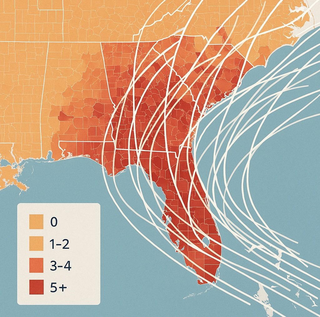
During the last 49 years, 338 hurricanes have struck 640 counties within the southeastern US. Coastal counties bear the brunt of wind and storm surge, whereas inland areas endure from torrential rain and the occasional hurricane-spawned twister. It’s a posh, far-reaching hazard, and with the fitting instruments, you may map it county by county.

The next map, constructed utilizing the Tropycal library, information the tracks of all of the hurricanes that made landfall within the US from 1975 by way of 2024.

Whereas attention-grabbing, this map isn’t a lot use to an insurance coverage adjuster. We have to quantify it by including county-level decision and counting the variety of distinctive tracks that cross into every county. Right here’s how that appears:

Now we’ve a greater thought of which counties act as “hurricane magnets.” Throughout the Southeast, hurricane “hit” counts vary from zero to 12 per county — however the storms are removed from evenly distributed. Hotspots cluster alongside the Louisiana coast, in central Florida, and alongside the shorelines of the Carolinas. The East Coast actually takes it on the chin, with Brunswick County, North Carolina, holding the unwelcome report for essentially the most hurricane strikes.

A look on the monitor map makes the sample clear. Florida, Georgia, South Carolina, and North Carolina sit within the crosshairs of two storm highways — one from the Atlantic and one other from the Gulf of Mexico. The prevailing westerlies, which start simply north of the Gulf Coast, usually bend northward-tracking storms towards the Atlantic seaboard. Fortuitously for Georgia and the Carolinas, many of those programs lose power over land, slipping under hurricane power earlier than sweeping by way of.

For insurers, these visualizations aren’t simply climate curiosities; they’re decision-making instruments. And layering in historic loss information can present a extra full image of the true monetary value of dwelling by the water’s edge.

The Choropleth Code

The next code, written in JupyterLab, creates a choropleth map of hurricane monitor counts per county. It makes use of geospatial information from the Plotly graphing library and pulls open-source climate information from the Nationwide Oceanic and Atmospheric Administration (NOAA) utilizing the Tropycal library.

The code makes use of the next packages:

python 3.10.18
numpy 2.2.5
geopandas 1.0.1
plotly 6.0.1 (plotly_express 0.4.1)
tropical 1.4
shapely 2.0.6

Importing Libraries

Begin by importing the next libraries.

import json
import numpy as np
import geopandas as gpd
import plotly.specific as px
from tropycal import tracks
from shapely.geometry import LineString

Configuring Constants

Now, we arrange a number of constants. The primary is a set of the state “FIPS” codes. Brief for Federal Data Processing Sequence, these “zip codes for states” are generally utilized in geospatial recordsdata. On this case, they characterize the southeastern states of Alabama, Florida, Georgia, Louisiana, Mississippi, North Carolina, South Carolina, and Texas. Later, we’ll use these codes to filter a single file of all the USA.

# CONFIGURE CONSTANTS
# State: AL, FL, GA, LA, MS, NC, SC, TX:
SE_STATE_FIPS = {'01', '12', '13', '22', '28', '37', '45', '48'}  
YEAR_RANGE = (1975, 2024)
INTENSITY_THRESH = {'v_min': 64}  # Hurricanes (>= 64 kt)
COUNTY_GEOJSON_URL = (
 'https://uncooked.githubusercontent.com/plotly/datasets/grasp/geojson-counties-fips.json'
)

Subsequent, we outline a 12 months vary (1975-2024) as a tuple. Then, we assign an depth threshold fixed for wind velocity. Tropycal will filter storms based mostly on wind speeds, and people with speeds of 64 knots or larger are categorized as hurricanes.

Lastly, we offer the URL handle for the Plotly library’s counties geospatial shapefile. Later, we’ll use GeoPandas to load this as a GeoDataFrame, which is basically a pandas DataFrame with a Geometry column for geospatial mapping data.

NOTE: Hurricanes rapidly turn into tropical storms and depressions after making landfall. These are nonetheless damaging, nevertheless, so we’ll proceed to trace them.

Defining Helper Features

To streamline the hurricane mapping workflow, we’ll outline three light-weight helper capabilities. These will assist hold the code modular, readable, and adaptable, particularly when working with real-world geospatial information that will range in construction or scale.

# Outline Helper Features:
def get_hover_name_column(df: gpd.GeoDataFrame) -> str:
    # Favor proper-case county title if obtainable:
    if 'NAME' in df.columns:
        return 'NAME'
    if 'title' in df.columns:
        return 'title'
    # Fallback to id if no title column exists:
    return 'id'

def storm_to_linestring(storm_obj) -> LineString | None:
    df = storm_obj.to_dataframe()
    if len(df) < 2:
        return None
    coords = [(lon, lat) for lon, lat in zip(df['lon'], df['lat'])
              if not (np.isnan(lon) or np.isnan(lat))]
    return LineString(coords) if len(coords) > 1 else None

def make_tickvals(vmax: int) -> listing[int]:
    if vmax <= 10:
        step = 2
    elif vmax <= 20:
        step = 4
    elif vmax <= 50:
        step = 10
    else:
        step = 20
    return listing(vary(0, int(vmax) + 1, step)) or [0]

Plotly Specific creates interactive visuals. We’ll be capable to hover the cursor over counties within the choropleth map and launch a pop-up window of the county title and the variety of hurricanes which have handed by way of. The get_hover_name_column(df) perform selects essentially the most readable column title for map hover labels. It checks for 'NAME' or 'title' within the GeoDataFrame and defaults to 'id' if neither is discovered. This ensures constant labeling throughout datasets.

The storm_to_linestring(storm_obj) perform converts a storm’s monitor information right into a LineString geometry by extracting legitimate longitude–latitude pairs. If the storm has fewer than two legitimate factors, it returns ‘None’. That is important for spatial joins and visualizing storm paths.

Lastly, the make_tickvals(vmax) perform generates a clear set of tick marks for the choropleth colorbar based mostly on the utmost hurricane rely. It dynamically adjusts the step dimension to maintain the legend readable, whether or not the vary is small or massive.

Put together the County Map

The subsequent cell masses the geospatial information and filters out the southeastern states, utilizing our ready set of FIPS codes. Within the course of, it creates a GeoDataFrame and provides a column for the Plotly Specific hover information.

# Load and filter county boundary information:
counties_gdf = gpd.read_file(COUNTY_GEOJSON_URL)

# Guarantee FIPS id is string with main zeros:
counties_gdf['id'] = counties_gdf['id'].astype(str).str.zfill(5)

# Derive state code from id's first two digits:
counties_gdf['STATE_FIPS'] = counties_gdf['id'].str[:2]
se_counties_gdf = (counties_gdf[counties_gdf['STATE_FIPS'].
                   isin(SE_STATE_FIPS)].copy())
hover_col = get_hover_name_column(se_counties_gdf)

print(f"Loading county information...")
print(f"Loaded {len(se_counties_gdf)} southeastern counties")

To start, we load the county-level GeoJSON file utilizing GeoPandas and put together it for evaluation. Every county is recognized by a FIPS code, which we format as a 5-digit string to make sure consistency (the primary two digits characterize the state code). We then extract the state portion of every FIPS code and filter the dataset to incorporate solely counties in our eight southeastern states. Lastly, we choose a column for labeling counties within the hover textual content and make sure the variety of counties which have been loaded.

Fetching and Processing Hurricane Information

Now it’s time to make use of Tropycal to fetch and course of the hurricane information from the Nationwide Hurricane Heart. That is the place we programmatically overlay the counties with the hurricane tracks and rely the distinctive occurrences of tracks in every county.

# Get and course of hurricane information utilizing Tropycal library:
strive:
    atlantic = tracks.TrackDataset(basin='north_atlantic', 
                                   supply='hurdat', 
                                   include_btk=True)

    storms_ids = atlantic.filter_storms(thresh=INTENSITY_THRESH,
                                                  year_range=YEAR_RANGE)

    print(f"Discovered {len(storms_ids)} hurricanes from "
    f"{YEAR_RANGE[0]}–{YEAR_RANGE[1]}")

    storm_names = []
    storm_tracks = []

    for i, sid in enumerate(storms_ids, begin=1):
        if i % 50 == 0 or i == 1 or i == len(storms_ids):
            print(f"Processing storm {i}/{len(storms_ids)}")
        strive:
            storm = atlantic.get_storm(sid)
            geom = storm_to_linestring(storm)
            if geom just isn't None:
                storm_tracks.append(geom)
                storm_names.append(storm.title)
        besides Exception as e:
            print(f"  Skipped {sid}: {e}")

    print(f"Efficiently processed {len(storm_tracks)} storm tracks")

    hurricane_tracks_gdf = gpd.GeoDataFrame({'title': storm_names}, 
                                            geometry=storm_tracks,
                                            crs="EPSG:4326")

    # Pre-filter tracks to the bounding field of the SE counties for velocity:
    xmin, ymin, xmax, ymax = se_counties_gdf.total_bounds
    hurricane_tracks_gdf = hurricane_tracks_gdf.cx[xmin:xmax, ymin:ymax]

    # Test that county information and hurricane tracks are similar CRS:
    assert se_counties_gdf.crs == hurricane_tracks_gdf.crs, 
    f"CRS mismatch: {se_counties_gdf.crs} vs {hurricane_tracks_gdf.crs}"

    # Spatial be part of to seek out counties intersecting hurricane tracks:
    print("Performing spatial be part of...")
    joined = gpd.sjoin(se_counties_gdf[['id', hover_col, 'geometry']],
                       hurricane_tracks_gdf[['name', 'geometry']],
                       how="internal",
                       predicate="intersects")

    # Rely distinctive hurricanes per county:
    unique_pairs = joined[['id', 'name']].drop_duplicates()
    hurricane_counts = (unique_pairs.groupby('id', as_index=False).dimension().
                                    rename(columns={'dimension': 'hurricane_count'}))

    # Merge counts again
    se_counties_gdf = se_counties_gdf.merge(hurricane_counts, 
                                            on='id', 
                                            how='left')
    se_counties_gdf['hurricane_count'] = (se_counties_gdf['hurricane_count'].
                                          fillna(0).astype(int))

    print(f"Hurricane counts: Max: {se_counties_gdf['hurricane_count'].max()} | "
          f"Nonzero counties: {(se_counties_gdf['hurricane_count'] > 0).sum()}")

besides Exception as e:
    print(f"Error loading hurricane information: {e}")
    print("Creating pattern information for demonstration...")
    np.random.seed(42)
    se_counties_gdf['hurricane_count'] = np.random.poisson(2, 
                                                           len(se_counties_gdf))

Right here’s a breakdown of the key steps:

• Load Dataset: Initializes the TrackDataset utilizing HURDAT information, together with greatest monitor (btk) factors.
• Filter Storms: Selects hurricanes that meet a specified depth threshold and fall inside a given 12 months vary.
• Extract Tracks: Iterates by way of every storm ID, converts its path to a LineString geometry, and shops each the monitor and storm title. Progress is printed each 50 storms.
• Create GeoDataFrame: Combines storm names and geometries right into a GeoDataFrame with WGS84 coordinates.
• Spatial Filtering: Clips hurricane tracks to the bounding field of southeastern counties to enhance efficiency.
• Assert CRS: Checks that the county and hurricane information use the identical coordinate reference system (in case you need to use totally different geospatial and/or hurricane monitor recordsdata).
• Spatial Be a part of: Identifies which counties intersect with hurricane tracks utilizing a spatial be part of.

Performing the spatial be part of might be tough. For instance, if a monitor doubles again and re-enters a county, you don’t need to rely it twice.

To deal with this, the code first identifies distinctive title pairs after which drops duplicate rows from the GeoDataFrame earlier than performing the rely.

• Rely Hurricanes per County:
  • Drops duplicate storm–county pairs.
  • Teams by county ID to rely distinctive hurricanes.
  • Merges outcomes again into the county GeoDataFrame.
  • Fills lacking values with zero and converts to integer.
• Fallback Dealing with: If hurricane information fails to load, artificial hurricane counts are generated utilizing a Poisson distribution for demonstration functions. That is for studying the method, solely!

Errors loading the hurricane information are widespread, so keep watch over the printout. If the information fails to load, hold rerunning the cell till it does.

A profitable run will yield the next affirmation:

Constructing the Choropleth Map

The subsequent cell generates a personalized choropleth map of hurricane counts per county within the Southeastern US utilizing Plotly Specific.

# Construct the choropleth map:
print("Creating choropleth map...")

se_geojson = json.masses(se_counties_gdf.to_json())
max_count = int(se_counties_gdf['hurricane_count'].max())
tickvals  = make_tickvals(max_count)

fig = px.choropleth(se_counties_gdf, 
                    geojson=json.masses(se_counties_gdf.to_json()),
                    places='id',
                    featureidkey='properties.id',
                    coloration='hurricane_count',
                    color_continuous_scale='Reds',
                    range_color=[0, max_count],
                    title=(f"Southeastern US: Hurricane Counts Per County "
                           f"({YEAR_RANGE[0]}–{YEAR_RANGE[1]})"),
                    hover_name=hover_col,
                    hover_data={'hurricane_count': True, 'id': False})

# Regulate the map format and clear the Plotly hover information:
fig.update_geos(fitbounds="places", seen=False)
fig.update_traces(
    hovertemplate="%{hovertext}
Hurricanes: %{z}"
)

fig.update_layout(
    width=1400,
    peak=1000,
    title=dict(
        textual content=(f"Southeastern US: Hurricane Counts Per County "
              f"({YEAR_RANGE[0]}–{YEAR_RANGE[1]})"),
        x=0.5,
        xanchor='middle',
        y=0.85,
        yanchor='prime',
        font=dict(dimension=24),
        pad=dict(t=0, b=10)
    ),
    coloraxis_colorbar=dict(
        x=0.96,
        y=0.5,
        len=0.4,
        thickness=16,
        title='Hurricane Rely',
        outlinewidth=1,
        tickvals=tickvals,
        tickfont=dict(dimension=16)
    )
)

fig.add_annotation(
    textual content="Information: HURDAT2 by way of Tropycal | Metric: counties intersecting hurricane "
         f"tracks ({YEAR_RANGE[0]}–{YEAR_RANGE[1]})",
    x=0.521,
    y=0.89,
    showarrow=False,
    font=dict(dimension=16),
    xanchor='middle'
)

fig.present()

The important thing steps right here embody:

• GeoJSON Conversion: Converts the GeoDataFrame of counties to GeoJSON format for straightforward mapping with Plotly Specific.
• Colour Scaling: Determines the utmost hurricane rely and calls the helper perform to create tick values for the colorbar.
• Map Rendering:
  • Makes use of px.choropleth to visualise hurricane_count per county.
    • The places='id' argument tells Plotly which column within the GeoDataFrame comprises the distinctive identifiers for every county (county-level FIPS codes). These values match every row of information to the corresponding form within the GeoJSON file.
    • The featureidkey='properties.id' argument specifies the place to seek out the matching identifier contained in the GeoJSON construction. GeoJSON options have a properties dictionary containing an 'id' discipline. This ensures that every county’s geometry is appropriately paired with its hurricane rely.
    • Applies a crimson coloration scale, units the vary, and defines hover conduct.
• Structure & Styling:
  • Facilities and kinds the title.
  • Adjusts map bounds and hides geographic outlines.
    • The fig.update_geos(fitbounds="places", seen=False) line turns off the bottom map for a cleaner plot.
  • Refines hover tooltips for readability.
  • Customizes the colorbar with tick marks and labels.
• Annotation: Provides an information supply word referencing HURDAT2 and the evaluation metric.
• Show: Reveals the ultimate interactive map with fig.present().

The deciding consider utilizing Plotly Specific over static instruments like Matplotlib is the addition of the dynamic hover information. Since there’s no sensible option to label a whole lot of counties, the hover information helps you to question the map whereas conserving all that additional data out of sight till wanted.

The Observe Map Code

Though pointless, viewing the precise hurricane tracks can be a pleasant contact, in addition to a option to verify the choropleth outcomes. This map might be generated fully with the Tropycal library, as proven under.

# Plot tracks coloured by class:
title = 'SE USA Hurricanes (1975-2024)'
ax = atlantic.plot_storms(storms=storms_ids,
                          title=title,
                          area={'w':-97.68,'e':-70.3,'s':22,'n':ymax},
                          prop={'plot_names':False, 
                                'dots':False,
                                'linecolor':'class',
                                'linewidth':1.0}, 
                          map_prop={'plot_gridlines':False})

# plt.savefig('counties_tracks.png', dpi=600, bbox_inches='tight')

Notice that the area parameter refers back to the boundaries of the map. Whereas you should use our earlier xmin, xmax, ymin, and ymax variables, I’ve adjusted them barely for a extra visually interesting map. Right here’s the outcome:

For extra on utilizing the Tropycal library, see my earlier article: Simple Hurricane Monitoring with Tropycal | by Lee Vaughan | TDS Archive | Medium.

The Hurricane Record Code

No insurance coverage adjuster will need to cursor by way of a map to extract information. As a result of GeoDataFrames are a type of pandas DataFrame, it’s straightforward to slice and cube the information and current it as tables. The next code types the counties by hurricane rely after which, for brevity, shows the highest 20 counties based mostly on their rely.

Right here’s the fast and simple option to generate this desk; I’ve added some additional code for the state abbreviations:

# Map FIPS to state abbreviation:
fips_to_abbrev = {'01': 'AL', '12': 'FL', '13': 'GA', '22': 'LA', 
                  '28': 'MS', '37': 'NC', '45': 'SC', '48': 'TX'}

# Add state abbreviation column:
se_counties_gdf['state_abbrev'] = se_counties_gdf['STATE'].map(fips_to_abbrev)

# Type and choose prime 20 counties by hurricane rely
top20 = (se_counties_gdf.sort_values(by='hurricane_count', 
                                     ascending=False) 
         [['state_abbrev', 'NAME', 'hurricane_count']].head(20))

# Show outcome
print(top20.to_string(index=False))

And right here’s the outcome:

Whereas this works, it’s not very professional-looking. We will enhance it utilizing an HTML strategy:

# Print out the highest 20 counties based mostly on hurricane impacts:
# Map FIPS to state abbreviation:
fips_to_abbrev = {'01': 'AL', '12': 'FL', '13': 'GA', '22': 'LA', 
                  '28': 'MS', '37': 'NC', '45': 'SC', '48': 'TX'}

gdf_sorted = se_counties_gdf.copy()

# Add new column for state abbreviation:
gdf_sorted['State Name'] = gdf_sorted['STATE'].map(fips_to_abbrev)

# Rename Current Columns:
# A number of columns without delay
gdf_sorted = gdf_sorted.rename(columns={'NAME': 'County Title', 
                                        'hurricane_count': 'Hurricane Rely'})

# Type by hurricane_count:
gdf_sorted = gdf_sorted.sort_values(by='Hurricane Rely', ascending=False)

# Create a pretty HTML show:
df_display = gdf_sorted[['State Name', 'County Name', 'Hurricane Count']].head(20)
df_display['Hurricane Count'] = df_display['Hurricane Count'].astype(int)

# Create styled HTML desk with out index:
styled_table = (
    df_display
        .fashion
        .set_caption("Prime 20 Counties by Hurricane Impacts")
        .set_table_styles([
            # Hide the index
            {'selector': 'th.row_heading',
             'props': [('display', 'none')]},
            {'selector': 'th.clean',
             'props': [('display', 'none')]},

            # Caption styling:
            {'selector': 'caption',
             'props': [('caption-side', 'top'),
                       ('font-size', '16px'),
                       ('font-weight', 'bold'),
                       ('text-align', 'center'),
                       ('color', '#333')]},

            # Header styling:
            {'selector': 'th.col_heading',
             'props': [('background-color', '#004466'),
                       ('color', 'white'),
                       ('text-align', 'center'),
                       ('padding', '6px')]},

            # Cell styling:
            {'selector': 'td',
             'props': [('text-align', 'center'),
                       ('padding', '6px')]}
        ])
        # Add zebra striping:
        .apply(lambda col: [
            'background-color: #f2f2f2' if i % 2 == 0 else ''
            for i in range(len(col))
        ], axis=0)
)

# Save styled HTML desk to disk:
styled_table.to_html("top20_hurricane_table.html")
styled_table

This cell transforms our uncooked geospatial information right into a clear, publication-ready abstract of hurricane publicity by county. It prepares and presents a ranked desk of the 20 counties most affected by hurricanes:

• State Abbreviation Mapping: It begins by mapping every county’s FIPS state code to its two-letter abbreviation (e.g., '48' → 'TX') and provides this as a brand new column.
• Column Renaming: The county title ('NAME') and hurricane rely ('hurricane_count') columns are renamed to 'County Title' and 'Hurricane Rely' for readability.
• Sorting and Choice: The GeoDataFrame is sorted in descending order by hurricane rely, and the highest 20 rows are chosen.
• Styled Desk Creation: Utilizing pandas’ Styler, the code builds a visually formatted HTML desk:
  • Provides a centered caption
  • Hides the index column
  • Applies customized header and cell styling
  • Provides zebra striping for readability
• Export to HTML: The styled desk is saved as top20_hurricane_table.html, making it straightforward to embed in stories or share externally.

Right here’s the outcome:

This desk might be additional enhanced by together with interactive sorting or by embedding it immediately right into a dashboard.

Abstract

On this venture, we addressed a query on each actuary’s desk: Which counties get hit the toughest by hurricanes, 12 months after 12 months? Python’s wealthy ecosystem of third-party packages was key to creating this straightforward and efficient. Tropycal made accessing authorities hurricane information a breeze, Plotly supplied the county boundaries, and GeoPandas merged the 2 datasets and counted the variety of hurricanes per county. Lastly, Plotly Specific produced a dynamic, interactive map that made it straightforward to visualise and discover the county-level hurricane information.