


Linear Regression, lastly!
For Day 11, I waited many days to current this mannequin. It marks the start of a new journey on this “Introduction Calendar“.
Till now, we largely checked out fashions primarily based on distances, neighbors, or native density. As it’s possible you’ll know, for tabular knowledge, determination bushes, particularly ensembles of determination bushes, are very performant.
However beginning right now, we change to a different perspective: the weighted method.
Linear Regression is our first step into this world.
It seems easy, however it introduces the core components of recent ML: loss features, gradients, optimization, scaling, collinearity, and interpretation of coefficients.
Now, after I say, Linear Regression, I imply Strange Least Sq. Linear Regression. As we progress by way of this “Introduction Calendar” and discover associated fashions, you will note why it is very important specify this, as a result of the title “linear regression” could be complicated.
Some folks say that Linear Regression is not machine studying.
Their argument is that machine studying is a “new” discipline, whereas Linear Regression existed lengthy earlier than, so it can’t be thought-about ML.
That is deceptive.
Linear Regression suits completely inside machine studying as a result of:
- it learns parameters from knowledge,
- it minimizes a loss operate,
- it makes predictions on new knowledge.
In different phrases, Linear Regression is among the oldest fashions, but in addition one of many most basic in machine studying.
That is the method utilized in:
- Linear Regression,
- Logistic Regression,
- and, later, Neural Networks and LLMs.
For deep studying, this weighted, gradient-based method is the one that’s used in all places.
And in trendy LLMs, we’re not speaking about just a few parameters. We’re speaking about billions of weights.
On this article, our Linear Regression mannequin has precisely 2 weights.
A slope and an intercept.
That’s all.
However we now have to start someplace, proper?
And listed below are just a few questions you may take into accout as we progress by way of this text, and within the ones to come back.
- We are going to attempt to interpret the mannequin. With one function, y=ax+b, everybody is aware of {that a} is the slope and b is the intercept. However how can we interpret the coefficients the place there are 10, 100 or extra options?
- Why is collinearity between options such an issue for linear regression? And the way can we do to resolve this challenge?
- Is scaling essential for linear regression?
- Can Linear regression be overfitted?
- And the way are the opposite fashions of this weighted familly (Logistic Regression, SVM, Neural Networks, Ridge, Lasso, and so on.), all linked to the identical underlying concepts?
These questions kind the thread of this text and can naturally lead us towards future subjects within the “Introduction Calendar”.
Understanding the Development line in Excel
Beginning with a Easy Dataset
Allow us to start with a quite simple dataset that I generated with one function.
Within the graph beneath, you may see the function variable x on the horizontal axis and the goal variable y on the vertical axis.
The purpose of Linear Regression is to seek out two numbers, a and b, such that we are able to write the connection:
y=a x +b
As soon as we all know a and b, this equation turns into our mannequin.

Creating the Development Line in Excel
In Google Sheets or Excel, you may merely add a pattern line to visualise one of the best linear match.
That already provides you the results of Linear Regression.

However the function of this text is to compute these coefficients ourselves.
If we wish to use the mannequin to make predictions, we have to implement it immediately.

Introducing Weights and the Price Operate
A Word on Weight-Based mostly Fashions
That is the primary time within the Introduction Calendar that we introduce weights.
Fashions that be taught weights are sometimes referred to as parametric discriminant fashions.
Why discriminant?
As a result of they be taught a rule that immediately separates or predicts, with out modeling how the information was generated.
Earlier than this chapter, we already noticed fashions that had parameters, however they weren’t discriminant, they had been generative.
Allow us to recap shortly.
- Resolution Bushes use splits, or guidelines, and so there are not any weights to be taught. So they’re non-parametric fashions.
- k-NN is just not a mannequin. It retains the entire dataset and makes use of distances at prediction time.
Nonetheless, once we transfer from Euclidean distance to Mahalanobis distance, one thing fascinating occurs…
LDA and QDA do estimate parameters:
- means of every class
- covariance matrices
- priors
These are actual parameters, however they don’t seem to be weights.
These fashions are generative as a result of they mannequin the density of every class, after which use it to make predictions.
So although they’re parametric, they don’t belong to the weight-based household.
And as you may see, these are all classifiers, and so they estimate parameters for every class.

Linear Regression is our first instance of a mannequin that learns weights to construct a prediction.
That is the start of a brand new household within the Introduction Calendar:
fashions that depend on weights + a loss operate to make predictions.
The Price Operate
How can we acquire the parameters a and b?
Effectively, the optimum values for a and b are these minimizing the associated fee operate, which is the Squared Error of the mannequin.
So for every knowledge level, we are able to calculate the Squared Error.
Squared Error = (prediction-real worth)²=(a*x+b-real worth)²
Then we are able to calculate the MSE, or Imply Squared Error.
As we are able to see in Excel, the trendline provides us the optimum coefficients. When you manually change these values, even barely, the MSE will enhance.
That is precisely what “optimum” means right here: another mixture of a and b makes the error worse.

The basic closed-form answer
Now that we all know what the mannequin is, and what it means to reduce the squared error, we are able to lastly reply the important thing query:
How can we compute the 2 coefficients of Linear Regression, the slope a and the intercept b?
There are two methods to do it:
- the precise algebraic answer, generally known as the closed-form answer,
- or gradient descent, which we’ll discover simply after.
If we take the definition of the MSE and differentiate it with respect to a and b, one thing lovely occurs: every little thing simplifies into two very compact formulation.

These formulation solely use:
- the common of x and y,
- how x varies (its variance),
- and the way x and y fluctuate collectively (their covariance).
So even with out realizing any calculus, and with solely fundamental spreadsheet features, we are able to reproduce the precise answer utilized in statistics textbooks.
interpret the coefficients
For one function, interpretation is easy and intuitive:
The slope a
It tells us how a lot y modifications when x will increase by one unit.
If the slope is 1.2, it means:
“when x goes up by 1, the mannequin expects y to go up by about 1.2.”
The intercept b
It’s the predicted worth of y when x = 0.
Typically, x = 0 doesn’t exist in the true context of the information, so the intercept is just not all the time significant by itself.
Its position is generally to place the road appropriately to match the middle of the information.
That is often how Linear Regression is taught:
a slope, an intercept, and a straight line.
With one function, interpretation is straightforward.
With two, nonetheless manageable.
However as quickly as we begin including many options, it turns into tougher.
Tomorrow, we’ll focus on additional concerning the interpretation.
In the present day, we’ll do the gradient descent.
Gradient Descent, Step by Step
After seeing the basic algebraic answer for Linear Regression, we are able to now discover the opposite important device behind trendy machine studying: optimization.
The workhorse of optimization is Gradient Descent.
Understanding it on a quite simple instance makes the logic a lot clearer as soon as we apply it to Linear Regression.
A Mild Heat-Up: Gradient Descent on a Single Variable
Earlier than implementing the gradient descent for the Linear Regression, we are able to first do it for a easy operate: (x-2)^2.
Everybody is aware of the minimal is at x=2.
However allow us to faux we have no idea that, and let the algorithm uncover it by itself.
The thought is to seek out the minimal of this operate utilizing the next course of:
- First, we randomly select an preliminary worth.
- Then for every step, we calculate the worth of the by-product operate df (for this x worth): df(x)
- And the subsequent worth of x is obtained by subtracting the worth of by-product multiplied by a step dimension: x = x – step_size*df(x)
You may modify the 2 parameters of the gradient descent: the preliminary worth of x and the step dimension.
Sure, even with 100, or 1000. That’s fairly shocking to see, how effectively it really works.

However, in some circumstances, the gradient descent won’t work. For instance, if the step dimension is just too huge, the x worth can explode.

Gradient descent for linear regression
The precept of the gradient descent algorithm is similar for linear regression: we now have to calculate the partial derivatives of the associated fee operate with respect to the parameters a and b. Let’s notice them as da and db.
Squared Error = (prediction-real worth)²=(a*x+b-real worth)²
da=2(a*x+b-real worth)*x
db=2(a*x+b-real worth)

After which, we are able to do the updates of the coefficients.

With this tiny replace, step-by-step, the optimum worth will likely be discovered after just a few interations.
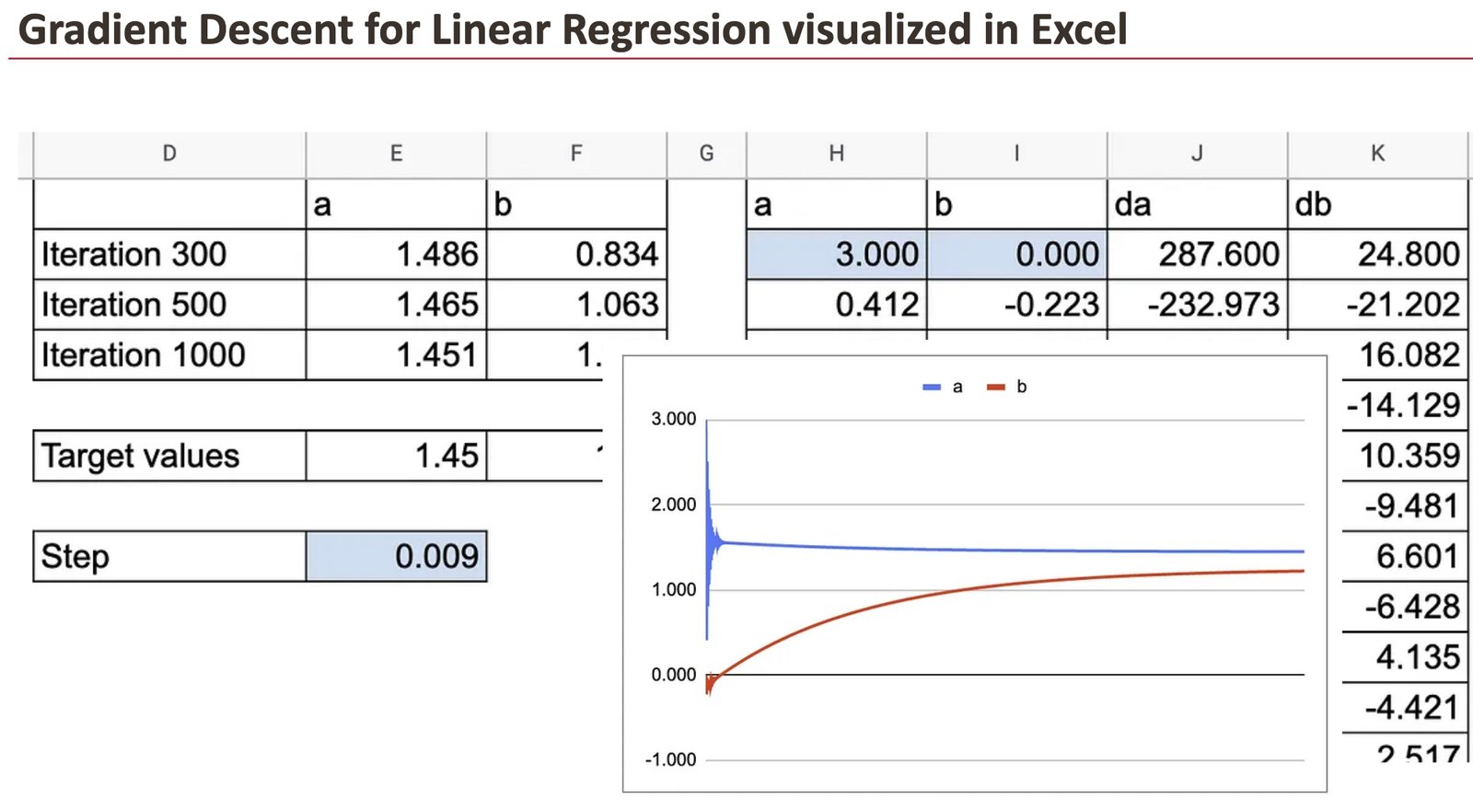
Within the following graph, you may see how a and b converge in the direction of the goal worth.

We will additionally see all the small print of y hat, residuals and the partial derivatives.
We will absolutely admire the great thing about gradient descent, visualized in Excel.
For these two coefficients, we are able to observe how fast the convergence is.

Now, in apply, we now have many observations and this ought to be accomplished for every knowledge level. That’s the place issues grow to be loopy in Google Sheet. So, we use solely 10 knowledge factors.
You will note that I first created a sheet with lengthy formulation to calculate da and db, which comprise the sum of the derivatives of all of the observations. Then I created one other sheet to point out all the small print.
Categorical Options in Linear Regression
Earlier than concluding, there’s one final essential concept to introduce:
how a weight-based mannequin like Linear Regression handles categorical options.
This subject is crucial as a result of it reveals a basic distinction between the fashions we studied earlier (like k-NN) and the weighted fashions we’re coming into now.
Why distance-based fashions wrestle with classes
Within the first a part of this Introduction Calendar, we used distance-based fashions similar to Ok-NN, DBSCAN, and LOF.
However these fashions rely solely on measuring distances between factors.
For categorical options, this turns into unimaginable:
- a class encoded as 0 or 1 has no quantitative which means
- the numerical scale is unfair,
- Euclidean distance can not seize class variations.
Because of this k-NN can not deal with classes appropriately with out heavy preprocessing.
Weight-based fashions resolve the issue in a different way
Linear Regression doesn’t examine distances.
It learns weights.
To incorporate a categorical variable in a weight-based mannequin, we use one-hot encoding, the commonest method.
Every class turns into its personal function, and the mannequin merely learns one weight per class.
Why this works so effectively
As soon as encoded:
- the dimensions downside disappears (every little thing is 0 or 1),
- every class receives an interpretable weight,
- the mannequin can modify its prediction relying on the group
A easy two-category instance
When there are solely two classes (0 and 1), the mannequin turns into very simple:
- one worth is used when x=0,
- one other when x=1.
One-hot encoding is just not even needed:
the numeric encoding already works as a result of Linear Regression will be taught the suitable distinction between the 2 teams.

Gradient Descent nonetheless works
Even with categorical options, Gradient Descent works precisely as typical.
The algorithm solely manipulates numbers, so the replace guidelines for a and b are an identical.
Within the spreadsheet, you may see the parameters converge easily, similar to with numerical knowledge.
Nonetheless, on this particular two-category case, we additionally know {that a} closed-form method exists: Linear Regression primarily computes two group averages and the distinction between them.

Conclusion
Linear Regression could look easy, however it introduces nearly every little thing that trendy machine studying depends on.
With simply two parameters, a slope and an intercept, it teaches us:
- the way to outline a value operate,
- the way to discover optimum parameters, numerically,
- and the way optimization behaves once we modify studying charges or preliminary values.
The closed-form answer reveals the magnificence of the arithmetic.
Gradient Descent reveals the mechanics behind the scenes.
Collectively, they kind the inspiration of the “weighted + loss operate” household that features Logistic Regression, SVM, Neural Networks, and even right now’s LLMs.
New Paths Forward
You could suppose Linear Regression is easy, however with its foundations now clear, you may lengthen it, refine it, and reinterpret it by way of many alternative views:
- Change the loss operate
Substitute squared error with logistic loss, hinge loss, or different features, and new fashions seem. - Transfer to classification
Linear Regression itself can separate two lessons (0 and 1), however extra strong variations result in Logistic Regression and SVM. And what about multiclass classification? - Mannequin nonlinearity
By polynomial options or kernels, linear fashions abruptly grow to be nonlinear within the authentic area. - Scale to many options
Interpretation turns into tougher, regularization turns into important, and new numerical challenges seem. - Primal vs twin
Linear fashions could be written in two methods. The primal view learns the weights immediately. The twin view rewrites every little thing utilizing dot merchandise between knowledge factors. - Perceive trendy ML
Gradient Descent, and its variants, are the core of neural networks and enormous language fashions.
What we realized right here with two parameters generalizes to billions.
All the pieces on this article stays inside the boundaries of Linear Regression, but it prepares the bottom for a complete household of future fashions.
Day after day, the Introduction Calendar will present how all these concepts join.


