Introduction
methods not often fail in a single second. Their efficiency adjustments regularly as information distributions shift, calibration drifts, or new patterns emerge within the surroundings. Ultimately the mannequin crosses a threshold the place it could possibly not be trusted. Most monitoring frameworks deal with this as a easy binary final result: the mannequin is both working or damaged. Right here we take a distinct perspective and deal with mannequin degradation as a time‑to‑failure drawback, and use instruments from survival evaluation and reliability engineering to quantify how lengthy a mannequin stays reliable after deployment.
Survival evaluation supplies a structured strategy to describe uncertainty over time. It helps reply questions equivalent to how lengthy a mannequin is predicted to final, how threat evolves as drift accumulates, and the way totally different mannequin households or deployment contexts evaluate when it comes to reliability. Ideas like survival curves, hazard features, and cumulative hazard have been initially developed for medical and industrial reliability, but they map naturally onto the lifecycle of ML methods. These instruments permit us to maneuver past advert hoc thresholds and towards principled, information‑pushed choices about retraining schedules, alerting insurance policies and lengthy‑time period upkeep.
This text is an excerpt from Chapter 8 of my new guide on Utilized Statistics for Knowledge Science, which is linked to on my website at qikly.com. All the photographs right here and in my guide have been created utilizing Python in Google Colab notebooks (my GitHub repository can be linked to by way of my website).
Contents
Half 1: Survival Evaluation for Machine Studying Reliability
- Survival Evaluation Necessities
- Weibull Distribution (β, η)
- Defining Time-to-Failure for ML Fashions
- Occasions and Censoring in ML Deployments
- Knowledge Drift and Distributional Shift
Half 2: Making use of Survival Estimators in Observe
- Simulated ML Reliability Dataset
- Drift‑Adjusted Weibull Failure Time Formulation
- Drift‑Adjusted Weibull Simulation
- Why Reliability Issues for ML Programs
- Actual Survival Dataset for Veteran Lung Most cancers
- Survival Curves and the Kaplan-Meier Estimator
- Survival Curves by Remedy Group
- Cumulative Hazard and the Nelson-Aalen Estimator
Half 3: Hazard-Based mostly Insights for ML Reliability
- Hazard-Based mostly Insights
- Spot‑Verify: Final Three Failures (Precise Hazard Values)
- Understanding Hazard Capabilities
- Growing older, Put on-Out and Failure Patterns
- Decoding Danger Over Time
- Abstract
1. Survival Evaluation for Machine Studying Reliability
Survival evaluation examines the timing of occasions and the variables that decide how lengthy methods, people, or fashions persist in a given state. It’s extensively utilized in medication, engineering, and machine studying to know time till failure, time till restoration, or time till a major change happens.
Survival Evaluation Necessities
The sphere contains foundational instruments such because the Kaplan–Meier estimator for survival curves and the Nelson–Aalen estimator for cumulative hazard.
A central concept in survival evaluation is the connection between the survival operate and the hazard operate. The survival operate describes the likelihood {that a} system or mannequin remains to be working at time t, whereas the hazard operate captures the instantaneous threat of failure at that very same second, on condition that the system has survived as much as time t. Collectively, these features present complementary views: survival tells us how lengthy methods final, and hazard tells us how threat evolves over time.

Weibull Distribution
The Weibull distribution is a versatile two‑parameter likelihood mannequin that performs a central position in reliability engineering, survival evaluation, and failure‑time modeling.
The Weibull distribution is extensively used as a result of it could possibly signify many several types of failure habits with solely a form parameter β and a scale parameter η.
Simulated Weibull Distributions (β, η)

– Within the left chart: η = 3 (scale is fastened) and β values are: [0.5, 1, 2, 5]
– In the precise chart: β = 2 (form is fastened) and η values are: [1, 2, 4, 6]
When β is lower than one, the hazard decreases over time, which corresponds to early‑life failures in engineering contexts and may also signify toddler mortality in sure medical research. When β equals one, the hazard is fixed, which corresponds to memoryless failure processes. When β is bigger than one, the hazard will increase over time, which corresponds to put on‑out, growing old, and degradation. This capability to seize reducing, fixed, or growing hazard patterns makes the Weibull distribution appropriate for mechanical methods, digital elements, and software program or ML fashions that deteriorate as their working situations change.
The dimensions parameter η units the attribute time scale of failure. Which means η determines the horizontal stretching of the distribution and establishes the standard lifetime of the system being modeled. A bigger worth of η shifts the distribution to the precise, which corresponds to longer anticipated lifetimes, whereas a smaller worth of η shifts it to the left, which corresponds to shorter anticipated lifetimes. In sensible phrases, η supplies a baseline measure of how lengthy a element or mannequin tends to operate earlier than failure happens, assuming no further accelerating elements equivalent to information drift or environmental stress.
It’s also mathematically handy as a result of it has a closed‑type density and cumulative distribution operate, and it helps easy inverse‑CDF sampling, which makes it ideally suited for simulation research.
Weibull Distribution Formulation

Defining Time-to-Failure for ML Fashions
Time-to-failure is the period of time a mannequin stays helpful earlier than its efficiency drops under a suitable stage. In apply, this threshold is tied to enterprise wants or security necessities. As soon as the mannequin falls under that stage, it’s thought-about to have failed even when it continues to provide outputs. Pondering when it comes to time to failure turns mannequin degradation right into a measurable amount that may be in contrast throughout fashions and used to plan retraining or alternative.
Occasions and Censoring in ML Deployments
In actual ML deployments, not each mannequin fails through the interval we observe it. Some fashions degrade sufficient to cross the failure threshold, and these are counted as occasions. Different fashions by no means attain that threshold earlier than monitoring ends, so they’re handled as censored. Censoring is widespread in apply as a result of fashions could also be changed early, retired for unrelated enterprise causes, or just not noticed lengthy sufficient to fail. In these circumstances, we solely know that the mannequin survived as much as its final statement time, and its eventual failure time stays unknown.
Distinguishing occasions from censored circumstances is important as a result of survival evaluation is designed to deal with this incomplete data with out bias.
Knowledge Drift and Distributional Shift
Knowledge drift refers to gradual adjustments within the enter distribution over time inside a given surroundings, whereas distributional shift describes the broader phenomenon wherein the info seen throughout deployment not matches the coaching distribution. Totally different deployments could drift quicker or slower relying on how shortly their native information evolves. Knowledge drift will not be the time‑to‑failure; it’s the fee at which the mannequin’s prediction high quality deteriorates as incoming information regularly shifts away from the distribution the mannequin was initially educated on.
2. Making use of Survival Estimators in Observe
We work with two kinds of datasets: a simulated reliability dataset generated utilizing the Weibull distribution, and an actual scientific dataset referred to as the Veteran Lung Most cancers Survival Dataset. These datasets permit us to discover each managed, mannequin‑pushed habits and actual‑world survival patterns.
Simulated ML Reliability Dataset
The purpose of the simulation is to create a practical reliability dataset for a single ML mannequin that’s deployed many occasions. Though the mannequin and its parameters are equivalent throughout deployments, every deployment experiences information drift at a distinct fee.
The failure mechanism is modeled with a Weibull distribution utilizing a form parameter β = 1.4 and a baseline scale η = 100. The form worth β larger than one produces an growing hazard over time, which simulates put on‑out and growing old. The baseline scale η units the standard failure time for a deployment with minimal drift.
To include information drift into the reliability simulation, every deployment is assigned a drift fee that determines how shortly its enter distribution adjustments over time. This drift fee is first remodeled right into a linear predictor, which scales proportionally with the drift fee and represents the power of the drift‑induced hazard improve. The linear predictor then modifies the Weibull scale parameter by means of an exponential transformation, producing an adjusted scale that turns into smaller as drift grows. A smaller scale compresses the failure‑time distribution towards earlier breakdowns. As soon as this adjusted scale is computed, the precise failure time is generated utilizing inverse‑CDF sampling from the Weibull distribution, which mixes the adjusted scale with the form parameter to provide sensible, drift‑dependent failure occasions.
Drift‑Adjusted Weibull Failure Time Formulation

Drift‑Adjusted Weibull Simulation
Simulation performs a vital position in ML reliability as a result of it lets us research failure habits below managed situations that mirror actual‑world degradation. By assigning drift charges, adjusting hazard phrases, and introducing censoring, we will observe how fashions fail, how threat accumulates, and the way monitoring home windows affect the habits of unpolluted, interpretable fashions. This type of artificial survival dataset is important for testing reliability strategies, validating hazard‑primarily based fashions, and understanding how drift and growing old work together lengthy earlier than failures happen in manufacturing.
Be aware within the above code that censoring is utilized by giving every deployment a random statement cutoff, which implies some fashions are nonetheless functioning when monitoring stops. Because of this, not each mannequin fails inside the interval we observe. Fashions that degrade sufficient to cross the failure threshold are counted as occasions, whereas those who by no means attain that threshold earlier than their cutoff are handled as censored.

Within the plots above, you’ll be able to see censoring immediately: failures focus at earlier occasions amongst excessive‑drift fashions, whereas censored deployments prolong to longer statement home windows the place monitoring stops earlier than the mannequin fails. Since drift drives the failure distribution, excessive‑drift fashions fail shortly and barely seem at lengthy noticed occasions, whereas low‑drift fashions survive lengthy sufficient to be censored.
Total, our simulation reveals how the ensuing dataset combines noticed occasions, occasion indicators, and drift values in a approach that captures a practical relationship between degradation fee and reliability.
Why Reliability Issues for ML Programs
Dependable habits is among the most vital qualities of any deployed mannequin as a result of choices made by downstream methods depend upon the mannequin remaining reliable over time.
The efficiency drift chart illustrates how reliability is assessed in apply. As an alternative of treating failure as an summary concept, the chart reveals the concrete alerts engineers monitor: the efficiency threshold that defines unacceptable habits, the second the mannequin truly crosses that line, and the restrict of the statement window. These visible cues flip mannequin degradation into one thing measurable and operational, getting ready the bottom for the reliability instruments launched in the remainder of the chapter.

The chart makes the affect of information drift straightforward to see: accuracy declines steadily till it falls under the efficiency threshold, marking the purpose the place the mannequin can not be thought-about dependable. We additionally see when the system is judged to have failed and the way lengthy it continues to be monitored afterward.
The essential values happen after accuracy drops under 0.75 and earlier than the failure level at roughly 0.73, comparable to occasions between about 72 and 80 days, which might have given monitoring personnel 8 days to take precautions. Be aware that the noticed time is just the size of the monitoring window, no matter whether or not the mannequin has already failed, as a result of efficiency continues to evolve after failure for the reason that mannequin remains to be operating and being measured.
Actual Survival Dataset for Veteran Lung Most cancers
To exhibit these strategies, we use information from the Veterans’ Administration Lung Most cancers Research, offered within the R survival bundle (Therneau, 2015), which is freely obtainable as open‑supply software program.
The dataset incorporates affected person‑stage observations collected throughout a scientific trial, and every row represents a single participant with a recorded survival time and an occasion indicator. The dataset contains each steady variables, equivalent to age and Karnofsky efficiency rating, and categorical variables, equivalent to therapy group and most cancers cell kind. These covariates permit for multivariable modeling utilizing Cox proportional hazards and Accelerated Failure Time (AFT) fashions. The survival occasions are measured in days, and the occasion indicator follows the usual conference the place one denotes loss of life and nil denotes censoring.

These plots present an outline of survival patterns, and each the distribution plot and the occasion‑day plot present that almost all sufferers have brief survival occasions, with loss of life occasions dominating early and censored circumstances showing far much less typically, primarily round 80 to 120 days.
Survival Curves and the Kaplan–Meier Estimator
The Kaplan–Meier estimator supplies a easy nonparametric strategy to estimate the likelihood of surviving past a given time whereas accounting for censored observations.

The Kaplan–Meier estimator is used as a result of it supplies a nonparametric estimate of the survival operate with out requiring any assumptions concerning the underlying distribution of occasion occasions. It incorporates censored observations in a pure approach, so people or methods that haven’t but skilled the occasion by the top of comply with‑up nonetheless contribute data. The ensuing curve is a stepwise estimate of survival that reveals how the likelihood of remaining occasion‑free adjustments at every noticed failure time.

Decoding the Kaplan–Meier curve is easy. The anticipated worth at any time t represents the estimated likelihood of surviving past that time. Every downward step within the curve corresponds to an noticed occasion, and the dimensions of the drop displays what number of failures occurred at the moment. Flat parts of the curve point out intervals with no noticed occasions. As a result of survival likelihood can’t improve as time progresses, the curve both stays flat or strikes downward, but it surely by no means rises.
Survival Curves by Remedy Group
The Veteran Lung Most cancers Survival Dataset contains two therapy teams that permit comparability of survival outcomes below totally different therapeutic methods. Sufferers have been assigned both an ordinary therapy or an experimental chemotherapy routine and the dataset information how lengthy every affected person survived after therapy started. These teams present a pure strategy to look at whether or not one strategy results in longer survival, how therapy interacts with affected person traits and the way survival curves can reveal variations in threat over time. By evaluating the Kaplan–Meier curves for every group, it turns into doable to see whether or not the experimental remedy affords any benefit or whether or not each remedies comply with comparable survival patterns.

To start with, as much as roughly 180 days, Remedy 1 (blue line) demonstrates a better survival likelihood in comparison with Remedy 2 (purple line). Nonetheless, after this essential threshold of 180 days, Remedy 2 maintains a considerably larger survival likelihood and sustained long-term efficacy for a for much longer period.
This intersection within the curves signifies a transition, with Remedy 1 providing higher speedy likelihood however Remedy 2 proving superior for general longevity.
Cumulative Hazard and the Nelson–Aalen Estimator
The Nelson–Aalen estimator supplies a nonparametric strategy to estimate the cumulative hazard operate by summing the noticed hazard contributions at every occasion time.

The Nelson–Aalen estimator is used as a result of it supplies a easy and sturdy strategy to estimate cumulative hazard with out assuming any specific distribution for occasion occasions. It incorporates censored observations by means of the chance set, so people or methods that stay occasion‑free nonetheless contribute details about how hazard accumulates. This estimator additionally serves as an vital hyperlink between hazard‑primarily based strategies and survival‑primarily based strategies, since cumulative hazard is among the elementary portions that connects the 2 views.

Decoding the Nelson–Aalen curve is easy. The anticipated worth at time t represents the whole accrued hazard skilled as much as that time. Bigger jumps within the curve happen at occasions with extra noticed occasions or when fewer people stay in danger. As a result of hazard accumulates quite than dissipates, the cumulative hazard curve all the time will increase over time and by no means decreases.
3. Hazard-Based mostly Insights for ML Reliability
Hazard-Based mostly Insights
The hazard operate affords a direct window into how the chance of failure adjustments as a system operates. As an alternative of compressing reliability right into a single lifetime estimate, it reveals whether or not the system is turning into extra fragile, extra steady, or staying fixed as time passes. For Machine Studying methods, this angle is very useful as a result of it highlights when fashions start to float, when information high quality deteriorates, or when operational stress begins to build up. By learning how the hazard evolves, groups can anticipate failures earlier than they happen and design interventions that hold methods reliable.

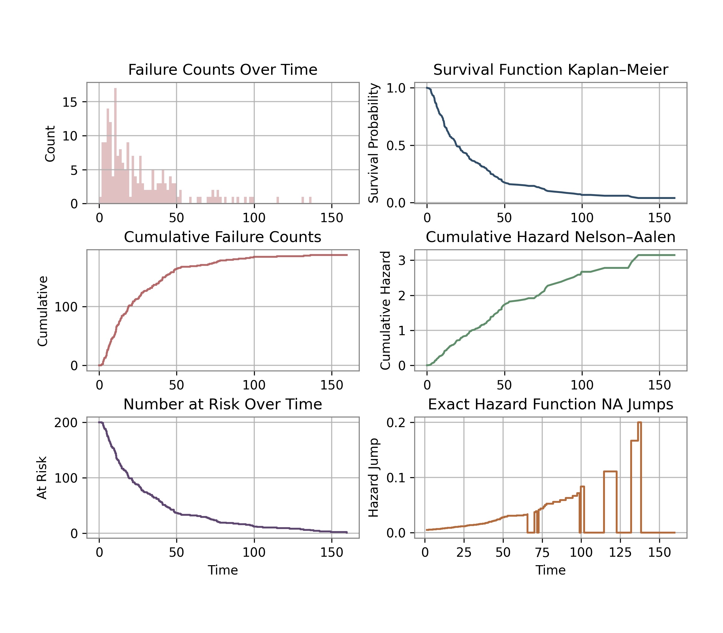
The gathering of plots comes from the simulated dataset and reveals a system transferring into a transparent put on‑out part. Failures grow to be extra concentrated at later occasions, the survival curve drops extra steeply, and the cumulative hazard accelerates. The quantity‑at‑threat curve thins quickly, and the precise hazard jumps develop bigger as fewer models stay, confirming that late‑stage failures carry considerably larger instantaneous threat. Collectively, the panels current a constant image of rising hazard because the inhabitants ages.
Spot‑Verify: Final Three Failures (Precise Hazard Values)
Subsequent, we spot‑verify the plotted information to make sure that the visible patterns actually come up from the underlying dataset quite than from plotting artifacts, indexing errors or workflow errors. On this spot‑verify, the final three failures present a centered view of how the system behaves close to the top of its lifetime, when solely a small variety of models stay in danger.

- The earliest of the final three failures happens when 9 models stay in danger, producing an actual hazard bounce of 0.1111, which displays a average per‑unit failure threat at that stage.
- The following failure occurs with solely 6 models nonetheless working, and the hazard bounce will increase to 0.1667, exhibiting that every remaining unit now carries a noticeably larger instantaneous threat.
- The ultimate failure happens when simply 5 models are left, and the hazard bounce rises additional to 0.2000, the most important bounce noticed, indicating a sharply elevated threat because the system approaches finish of life.
The steadily growing hazard jumps throughout these three occasions exhibit a transparent put on‑out sample, confirming that the late‑stage rise in hazard is significant and never an artifact of the estimator.
Understanding Hazard Capabilities
A hazard operate describes the instantaneous likelihood of failure at a selected second, on condition that the system has survived as much as that time. It captures the concept threat will not be uniform however will depend on age, surroundings and inside situations. A rising hazard signifies growing vulnerability, whereas a declining hazard suggests early instability adopted by stabilization. Flat areas present intervals of regular habits with no significant change in threat. For the reason that hazard operate is tied on to noticed occasion occasions, it supplies a transparent and interpretable strategy to perceive how threat accumulates and the way various factors form system habits.
Growing older, Put on-Out and Failure Patterns
Many methods comply with recognizable failure patterns that mirror underlying bodily or computational processes. Some fail early because of defects or unstable initialization, whereas others degrade slowly as elements put on down or as mannequin parameters drift from their unique calibration. Hazard evaluation makes these patterns seen by exhibiting whether or not threat is concentrated early, late, or unfold throughout the complete lifetime. This helps distinguish between early failures, random shocks, and true growing old results, permitting engineers to design upkeep schedules, retraining cycles, or monitoring methods that match the precise dynamics of failure.
Decoding Danger Over Time
Danger unfolds as a trajectory quite than a single worth and decoding it requires understanding how the hazard, survival and cumulative hazard features relate to 1 one other. The survival curve reveals the likelihood that the system stays operational, whereas the cumulative hazard reveals how a lot threat has accrued. The hazard operate reveals the native habits of threat at every second. When these views are mixed, they spotlight essential intervals the place intervention is simplest, reveal moments when the system turns into susceptible, and supply a basis for predictive upkeep and adaptive retraining. This time-based understanding of threat is important for constructing Machine Studying methods that stay dependable in actual world environments.
Abstract
We examined how survival evaluation supplies a sensible framework for managing the reliability of ML methods. We launched time‑to‑failure occasions that mirror actual deployment habits, constructed survival and hazard curves, and interpreted what these curves reveal about degradation patterns. We discovered interpret the 2 parameters of the Weibull distribution and the way they can be utilized to simulate drift‑adjusted Weibull failure time formulation. Utilized fashions equivalent to Kaplan–Meier and Nelson–Aalen have been demonstrated utilizing each actual and simulated datasets. Lastly, we noticed how hazard features assist establish when ML methods start to float, when information high quality deteriorates, and when operational stress begins to build up.
This text has coated the core concepts behind ML reliability. In case you’d prefer to discover these ideas additional, my new guide Utilized Statistics for Knowledge Science contains prolonged discussions of Cox fashions, Accelerated Failure Time (AFT) fashions, drift evaluation, and reliability‑primarily based monitoring methods. It’s obtainable at qikly.com.