Sesame  Speech Mannequin:  How This Viral AI Mannequin Generates Human-Like Speech

printed a demo of their newest Speech-to-Speech mannequin. A conversational AI agent who’s actually good at talking, they supply related solutions, they communicate with expressions, and actually, they’re simply very enjoyable and interactive to play with.

Be aware {that a} technical paper just isn’t out but, however they do have a quick weblog submit that gives quite a lot of details about the methods they used and former algorithms they constructed upon. 

Fortunately, they offered sufficient info for me to put in writing this text and make a YouTube video out of it. Learn on!

Coaching a Conversational Speech Mannequin

Sesame is a Conversational Speech Mannequin, or a CSM. It inputs each textual content and audio, and generates speech as audio. Whereas they haven’t revealed their coaching knowledge sources within the articles, we will nonetheless attempt to take a stable guess. The weblog submit closely cites one other CSM, 2024’s Moshi, and happily, the creators of Moshi did reveal their knowledge sources of their paper. Moshi makes use of 7 million hours of unsupervised speech knowledge, 170 hours of pure and scripted conversations (for multi-stream coaching), and 2000 extra hours of phone conversations (The Fischer Dataset).

However what does it actually take to generate audio?

In uncooked type, audio is only a lengthy sequence of amplitude values — a waveform. For instance, in case you’re sampling audio at 24 kHz, you might be capturing 24,000 float values each second.

In fact, it’s fairly resource-intensive to course of 24000 float values for only one second of knowledge, particularly as a result of transformer computations scale quadratically with sequence size. It could be nice if we may compress this sign and scale back the variety of samples required to course of the audio.

We’ll take a deep dive into the Mimi encoder and particularly Residual Vector Quantizers (RVQ), that are the spine of Audio/Speech modeling in Deep Studying right this moment. We’ll finish the article by studying about how Sesame generates audio utilizing its particular dual-transformer structure.

Preprocessing audio

Compression and have extraction are the place convolution helps us. Sesame makes use of the Mimi speech encoder to course of audio. Mimi was launched within the aforementioned Moshi paper as effectively. Mimi is a self-supervised audio encoder-decoder mannequin that converts audio waveforms into discrete “latent” tokens first, after which reconstructs the unique sign. Sesame solely makes use of the encoder part of Mimi to tokenize the enter audio tokens. Let’s learn the way.

Mimi inputs the uncooked speech waveform at 24Khz, passes them by means of a number of strided convolution layers to downsample the sign, with a stride issue of 4, 5, 6, 8, and a couple of. Which means the primary CNN block downsamples the audio by 4x, then 5x, then 6x, and so forth. In the long run, it downsamples by an element of 1920, lowering it to simply 12.5 frames per second.

The convolution blocks additionally undertaking the unique float values to an embedding dimension of 512. Every embedding aggregates the native options of the unique 1D waveform. 1 second of audio is now represented as round 12 vectors of measurement 512. This fashion, Mimi reduces the sequence size from 24000 to simply 12 and converts them into dense steady vectors.

What’s Audio Quantization?

Given the continual embeddings obtained after the convolution layer, we wish to tokenize the enter speech. If we will characterize speech as a sequence of tokens, we will apply normal language studying transformers to coach generative fashions.

Mimi makes use of a Residual Vector Quantizer or RVQ tokenizer to attain this. We’ll discuss concerning the residual half quickly, however first, let’s have a look at what a easy vanilla Vector quantizer does.

Vector Quantization

The concept behind Vector Quantization is straightforward: you practice a codebook , which is a group of, say, 1000 random vector codes all of measurement 512 (similar as your embedding dimension).

Then, given the enter vector, we’ll map it to the closest vector in our codebook — principally snapping a degree to its nearest cluster middle. This implies now we have successfully created a hard and fast vocabulary of tokens to characterize every audio body, as a result of regardless of the enter body embedding could also be, we’ll characterize it with the closest cluster centroid. If you wish to study extra about Vector Quantization, take a look at my video on this subject the place I am going a lot deeper with this.

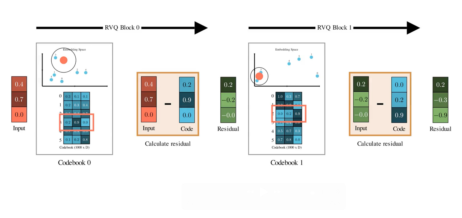
Residual Vector Quantization

The issue with easy vector quantization is that the lack of info could also be too excessive as a result of we’re mapping every vector to its cluster’s centroid. This “snap” isn’t excellent, so there may be at all times an error between the unique embedding and the closest codebook.

The massive thought of Residual Vector Quantization is that it doesn’t cease at having only one codebook. As an alternative, it tries to make use of a number of codebooks to characterize the enter vector.

1. First, you quantize the unique vector utilizing the primary codebook.
2. Then, you subtract that centroid out of your unique vector. What you’re left with is the residual — the error that wasn’t captured within the first quantization.
3. Now take this residual, and quantize it once more, utilizing a second codebook full of brand name new code vectors — once more by snapping it to the closest centroid.
4. Subtract that too, and also you get a smaller residual. Quantize once more with a 3rd codebook… and you may hold doing this for as many codebooks as you need.

Every step hierarchically captures slightly extra element that was missed within the earlier spherical. For those who repeat this for, let’s say, N codebooks, you get a group of N discrete tokens from every stage of quantization to characterize one audio body.

The best factor about RVQs is that they’re designed to have a excessive inductive bias in direction of capturing probably the most important content material within the very first quantizer. Within the subsequent quantizers, they study increasingly fine-grained options.

For those who’re acquainted with PCA, you may consider the primary codebook as containing the first principal elements, capturing probably the most important info. The next codebooks characterize higher-order elements, containing info that provides extra particulars.

Acoustic vs Semantic Codebooks

Since Mimi is skilled on the duty of audio reconstruction, the encoder compresses the sign to the discretized latent area, and the decoder reconstructs it again from the latent area. When optimizing for this activity, the RVQ codebooks study to seize the important acoustic content material of the enter audio contained in the compressed latent area. 

Mimi additionally individually trains a single codebook (vanilla VQ) that solely focuses on embedding the semantic content material of the audio. This is the reason Mimi known as a split-RVQ tokenizer – it divides the quantization course of into two unbiased parallel paths: one for semantic info and one other for acoustic info.

To coach semantic representations, Mimi used information distillation with an present speech mannequin known as WavLM as a semantic instructor. Principally, Mimi introduces an extra loss operate that decreases the cosine distance between the semantic RVQ code and the WavLM-generated embedding.

Audio Decoder

Given a dialog containing textual content and audio, we first convert them right into a sequence of token embeddings utilizing the textual content and audio tokenizers. This token sequence is then enter right into a transformer mannequin as a time sequence. Within the weblog submit, this mannequin is known as the Autoregressive Spine Transformer. Its activity is to course of this time sequence and output the “zeroth” codebook token.

A lighterweight transformer known as the audio decoder then reconstructs the following codebook tokens conditioned on this zeroth code generated by the spine transformer. Be aware that the zeroth code already incorporates quite a lot of details about the historical past of the dialog because the spine transformer has visibility of the complete previous sequence. The light-weight audio decoder solely operates on the zeroth token and generates the opposite N-1 codes. These codes are generated through the use of N-1 distinct linear layers that output the chance of selecting every code from their corresponding codebooks. 

You may think about this course of as predicting a textual content token from the vocabulary in a text-only LLM. Simply {that a} text-based LLM has a single vocabulary, however the RVQ-tokenizer has a number of vocabularies within the type of the N codebooks, so you could practice a separate linear layer to mannequin the codes for every.

Lastly, after the codewords are all generated, we mixture them to type the mixed steady audio embedding. The ultimate job is to transform this audio again to a waveform. For this, we apply transposed convolutional layers to upscale the embedding again from 12.5 Hz again to KHz waveform audio. Principally, reversing the transforms we had utilized initially throughout audio preprocessing.

In Abstract

So, right here is the general abstract of the Sesame mannequin in some bullet factors.

1.  Sesame is constructed on a multimodal Dialog Speech Mannequin or a CSM.
2. Textual content and audio are tokenized collectively to type a sequence of tokens and enter into the spine transformer that autoregressively processes the sequence.
3. Whereas the textual content is processed like some other text-based LLM, the audio is processed instantly from its waveform illustration. They use the Mimi encoder to transform the waveform into latent codes utilizing a cut up RVQ tokenizer.
4. The multimodal spine transformers eat a sequence of tokens and predict the following zeroth codeword.
5.  One other light-weight transformer known as the Audio Decoder predicts the following codewords from the zeroth codeword.
6. The ultimate audio body illustration is generated from combining all of the generated codewords and upsampled again to the waveform illustration.

Thanks for studying!

References and Should-read papers

Try my ML YouTube Channel

Sesame Blogpost and Demo

Related papers: 
Moshi: https://arxiv.org/abs/2410.00037 
SoundStream: https://arxiv.org/abs/2107.03312 
HuBert: https://arxiv.org/abs/2106.07447 
Speech Tokenizer: https://arxiv.org/abs/2308.16692