


On this article, you’ll learn to select between PCA and t-SNE for visualizing high-dimensional knowledge, with clear trade-offs, caveats, and dealing Python examples.
Matters we’ll cowl embody:
- The core concepts, strengths, and limits of PCA versus t-SNE.
- When to make use of every technique — and when to mix them.
- A sensible PCA → t-SNE workflow with scikit-learn code.
Let’s not waste any extra time.

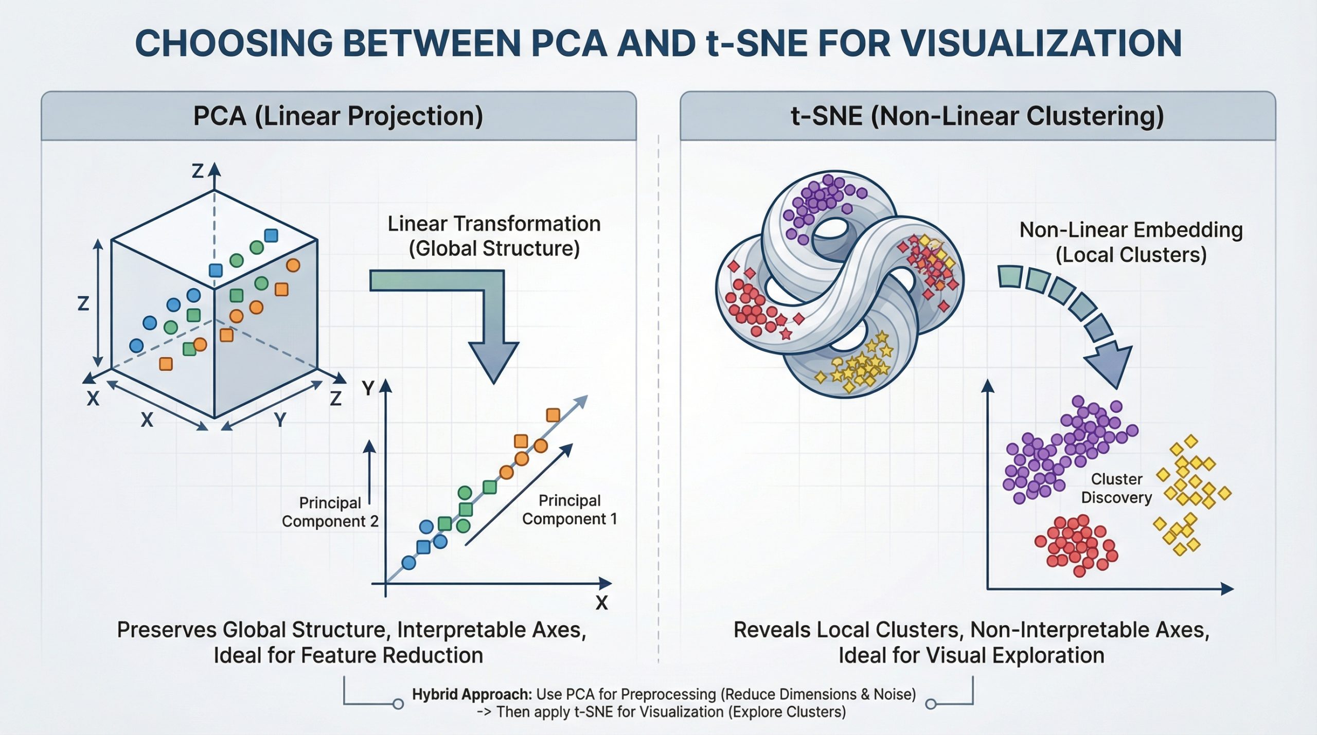
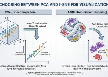
Selecting Between PCA and t-SNE for Visualization (click on to enlarge)
Picture by Editor
For knowledge scientists, working with high-dimensional knowledge is a part of day by day life. From buyer options in analytics to pixel values in pictures and phrase vectors in NLP, datasets typically comprise a whole lot and hundreds of variables. Visualizing such complicated knowledge is tough.
That’s the place dimensionality discount methods are available in. Two of probably the most extensively used strategies are Principal Part Evaluation (PCA) and t-Distributed Stochastic Neighbor Embedding (t-SNE). Whereas each scale back dimensions, they serve very totally different objectives.
Understanding Principal Part Evaluation (PCA)
Principal Part Evaluation is a linear technique that transforms knowledge into new axes known as principal elements. Its purpose is to transform your knowledge into a brand new coordinate system the place the best variations lie on the primary axis (the primary principal element), the second best on the second axis, and so forth. It does this by performing an eigendecomposition (the method of breaking down a sq. matrix into a less complicated, “canonical” kind utilizing its eigenvalues and eigenvectors) of the information covariance matrix or a Singular Worth Decomposition (SVD) of the information matrix.
These elements seize the best variance within the knowledge and are ordered from most essential to least essential. Consider PCA as rotating your dataset to search out the most effective angle that exhibits probably the most unfold of knowledge.
Key Benefits and When to Use PCA
- Function Discount & Preprocessing: Use PCA to cut back the variety of enter options for a downstream mannequin (like regression or classification) whereas retaining probably the most informative indicators.
- Noise Discount: By discarding elements with minor variance (typically noise), PCA can clear your knowledge.
- Interpretable Parts: You possibly can examine the
components_attribute to see which authentic options contribute most to every principal element. - World Variance Preservation: It faithfully maintains large-scale distances and relationships in your knowledge.
Implementing PCA with Scikit-Study
Utilizing PCA in Python’s scikit-learn is easy. The important thing parameter is n_components, which defines the variety of dimensions to your output.
|
1 2 3 4 5 6 7 8 9 10 11 12 13 14 15 16 17 18 19 20 21 22 23 24 25 |
from sklearn.decomposition import PCA from sklearn.datasets import load_iris import matplotlib.pyplot as plt
# Load pattern knowledge iris = load_iris() X = iris.knowledge y = iris.goal
# Apply PCA, decreasing to 2 dimensions for visualization pca = PCA(n_components=2) X_pca = pca.fit_transform(X)
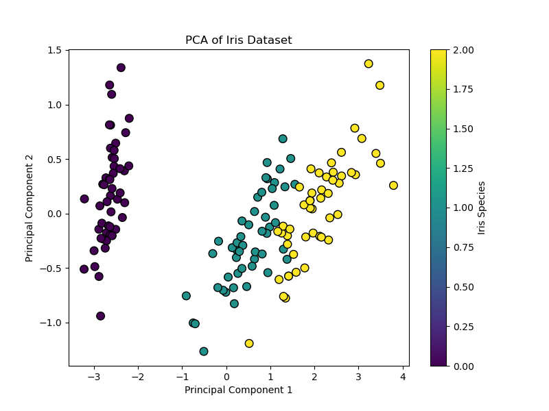
# Visualize the end result plt.determine(figsize=(8, 6)) scatter = plt.scatter(X_pca[:, 0], X_pca[:, 1], c=y, cmap=‘viridis’, edgecolor=‘okay’, s=70) plt.xlabel(‘Principal Part 1’) plt.ylabel(‘Principal Part 2’) plt.title(‘PCA of Iris Dataset’) plt.colorbar(scatter, label=‘Iris Species’) plt.present()
# Look at defined variance print(f“Variance defined by every element: {pca.explained_variance_ratio_}”) print(f“Complete variance captured: {sum(pca.explained_variance_ratio_):.2%}”) |
This code reduces the four-dimensional Iris dataset to 2 dimensions. The ensuing scatter plot exhibits the information unfold alongside axes of most variance, and the explained_variance_ratio_ tells you ways a lot data was preserved.
Code output:
|
Variance defined by every element: [0.92461872 0.05306648] Complete variance captured: 97.77% |
When to Use PCA
- Once you need to scale back options earlier than machine studying fashions
- Once you need to take away noise
- Once you need to pace up coaching
- Once you need to perceive world patterns
Understanding t-Distributed Stochastic Neighbor Embedding (t-SNE)
t-SNE is a non-linear method designed virtually fully for visualization. It really works by modeling pairwise similarities between factors within the high-dimensional house after which discovering a low-dimensional (2D or 3D) illustration the place these similarities are greatest maintained. It’s significantly good at revealing native constructions like clusters which may be hidden in excessive dimensions.
Key Benefits and When to Use t-SNE
- Visualizing Clusters: It’s nice for creating intuitive, cluster-rich plots from complicated knowledge like phrase embeddings, gene expression knowledge, or pictures
- Revealing Non-Linear Manifolds: It could actually reveal detailed, curved constructions that linear strategies like PCA can’t
- Concentrate on Native Relationships: Its design ensures that factors shut within the authentic house stay shut within the embedding
Vital Limitations
- Axes Are Not Interpretable: The t-SNE plot’s axes (t-SNE1, t-SNE2) haven’t any basic which means. Solely the relative distances and clustering of factors are informative
- Do Not Evaluate Clusters Throughout Plots: The dimensions and distances between clusters in a single t-SNE plot are usually not akin to these in one other plot from a distinct run or dataset
- Perplexity is Key: That is crucial parameter. It balances the eye between native and world construction (typical vary: 5–50). You have to experiment with it
Implementing t-SNE with Scikit-Study
|
1 2 3 4 5 6 7 8 9 10 11 12 13 14 15 16 17 18 19 20 21 |
from sklearn.datasets import load_iris from sklearn.manifold import TSNE import matplotlib.pyplot as plt
# Load pattern knowledge iris = load_iris() X = iris.knowledge y = iris.goal
# Apply t-SNE. Notice the important thing ‘perplexity’ parameter. tsne = TSNE(n_components=2, perplexity=30, random_state=42, init=‘pca’) X_tsne = tsne.fit_transform(X)
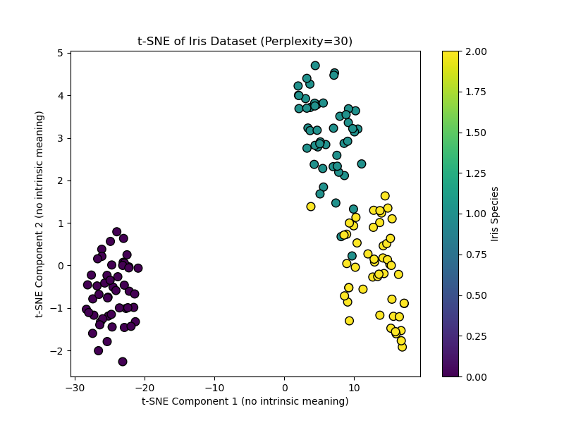
# Visualize the end result plt.determine(figsize=(8, 6)) scatter = plt.scatter(X_tsne[:, 0], X_tsne[:, 1], c=y, cmap=‘viridis’, edgecolor=‘okay’, s=70) plt.xlabel(‘t-SNE Part 1 (no intrinsic which means)’) plt.ylabel(‘t-SNE Part 2 (no intrinsic which means)’) plt.title(‘t-SNE of Iris Dataset (Perplexity=30)’) plt.colorbar(scatter, label=‘Iris Species’) plt.present() |
This code creates a t-SNE visualization. Setting init="pca" (the default) makes use of a PCA initialization for higher stability. Discover the axes are intentionally labeled as having no intrinsic which means.
Output:
When to Use t-SNE
- Once you need to discover clusters
- When you could visualize embeddings
- Once you need to reveal hidden patterns
- It isn’t for characteristic engineering
A Sensible Workflow
A strong and customary greatest follow is to mix PCA and t-SNE. This makes use of the strengths of each:
- First, use PCA to cut back very high-dimensional knowledge (e.g., 1000+ options) to an intermediate variety of dimensions (e.g., 50). This removes noise and drastically hastens the following t-SNE computation
- Then, apply t-SNE to the PCA output to get your ultimate 2D visualization
Hybrid method: PCA adopted by t-SNE
|
from sklearn.decomposition import PCA
# Step 1: Cut back to 50 dimensions with PCA pca_for_tsne = PCA(n_components=50) X_pca_reduced = pca_for_tsne.fit_transform(X_high_dim) # Assume X_high_dim is your authentic knowledge
# Step 2: Apply t-SNE to the PCA-reduced knowledge X_tsne_final = TSNE(n_components=2, perplexity=40, random_state=42).fit_transform(X_pca_reduced) |
The instance above demonstrates utilizing t-SNE to cut back to 2D for visualization, and the way PCA preprocessing could make t-SNE sooner and extra steady.
Conclusion
Choosing the proper software boils right down to your main goal:
- Use PCA whenever you want an environment friendly, deterministic, and interpretable technique for general-purpose dimensionality discount, characteristic extraction, or as a preprocessing step for an additional mannequin. It’s your go-to for a primary have a look at world knowledge construction.
- Use t-SNE when your purpose is solely visible exploration and cluster discovery in complicated, non-linear knowledge. Be ready to tune parameters and by no means interpret the plot quantitatively
Begin with PCA. If it reveals clear linear traits, it might be ample. In the event you suspect hidden clusters, swap to t-SNE (or use the hybrid method) to disclose them.
Lastly, whereas PCA and t-SNE are foundational, pay attention to trendy alternate options like Uniform Manifold Approximation and Projection (UMAP). UMAP is usually sooner than t-SNE and is designed to protect extra of the worldwide construction whereas nonetheless capturing native particulars. It has grow to be a preferred default alternative for a lot of visualization duties, persevering with the evolution of how we see our knowledge.
I hope this text supplies a transparent framework for selecting between PCA and t-SNE. The easiest way to construct this understanding is to experiment with each strategies on datasets you recognize effectively, observing how their totally different natures form the story your knowledge tells.
References
On this article, you’ll learn to select between PCA and t-SNE for visualizing high-dimensional knowledge, with clear trade-offs, caveats, and dealing Python examples.
Matters we’ll cowl embody:
- The core concepts, strengths, and limits of PCA versus t-SNE.
- When to make use of every technique — and when to mix them.
- A sensible PCA → t-SNE workflow with scikit-learn code.
Let’s not waste any extra time.
Selecting Between PCA and t-SNE for Visualization (click on to enlarge)
Picture by Editor
For knowledge scientists, working with high-dimensional knowledge is a part of day by day life. From buyer options in analytics to pixel values in pictures and phrase vectors in NLP, datasets typically comprise a whole lot and hundreds of variables. Visualizing such complicated knowledge is tough.
That’s the place dimensionality discount methods are available in. Two of probably the most extensively used strategies are Principal Part Evaluation (PCA) and t-Distributed Stochastic Neighbor Embedding (t-SNE). Whereas each scale back dimensions, they serve very totally different objectives.
Understanding Principal Part Evaluation (PCA)
Principal Part Evaluation is a linear technique that transforms knowledge into new axes known as principal elements. Its purpose is to transform your knowledge into a brand new coordinate system the place the best variations lie on the primary axis (the primary principal element), the second best on the second axis, and so forth. It does this by performing an eigendecomposition (the method of breaking down a sq. matrix into a less complicated, “canonical” kind utilizing its eigenvalues and eigenvectors) of the information covariance matrix or a Singular Worth Decomposition (SVD) of the information matrix.
These elements seize the best variance within the knowledge and are ordered from most essential to least essential. Consider PCA as rotating your dataset to search out the most effective angle that exhibits probably the most unfold of knowledge.
Key Benefits and When to Use PCA
- Function Discount & Preprocessing: Use PCA to cut back the variety of enter options for a downstream mannequin (like regression or classification) whereas retaining probably the most informative indicators.
- Noise Discount: By discarding elements with minor variance (typically noise), PCA can clear your knowledge.
- Interpretable Parts: You possibly can examine the
components_attribute to see which authentic options contribute most to every principal element. - World Variance Preservation: It faithfully maintains large-scale distances and relationships in your knowledge.
Implementing PCA with Scikit-Study
Utilizing PCA in Python’s scikit-learn is easy. The important thing parameter is n_components, which defines the variety of dimensions to your output.
|
1 2 3 4 5 6 7 8 9 10 11 12 13 14 15 16 17 18 19 20 21 22 23 24 25 |
from sklearn.decomposition import PCA from sklearn.datasets import load_iris import matplotlib.pyplot as plt
# Load pattern knowledge iris = load_iris() X = iris.knowledge y = iris.goal
# Apply PCA, decreasing to 2 dimensions for visualization pca = PCA(n_components=2) X_pca = pca.fit_transform(X)
# Visualize the end result plt.determine(figsize=(8, 6)) scatter = plt.scatter(X_pca[:, 0], X_pca[:, 1], c=y, cmap=‘viridis’, edgecolor=‘okay’, s=70) plt.xlabel(‘Principal Part 1’) plt.ylabel(‘Principal Part 2’) plt.title(‘PCA of Iris Dataset’) plt.colorbar(scatter, label=‘Iris Species’) plt.present()
# Look at defined variance print(f“Variance defined by every element: {pca.explained_variance_ratio_}”) print(f“Complete variance captured: {sum(pca.explained_variance_ratio_):.2%}”) |
This code reduces the four-dimensional Iris dataset to 2 dimensions. The ensuing scatter plot exhibits the information unfold alongside axes of most variance, and the explained_variance_ratio_ tells you ways a lot data was preserved.
Code output:
|
Variance defined by every element: [0.92461872 0.05306648] Complete variance captured: 97.77% |
When to Use PCA
- Once you need to scale back options earlier than machine studying fashions
- Once you need to take away noise
- Once you need to pace up coaching
- Once you need to perceive world patterns
Understanding t-Distributed Stochastic Neighbor Embedding (t-SNE)
t-SNE is a non-linear method designed virtually fully for visualization. It really works by modeling pairwise similarities between factors within the high-dimensional house after which discovering a low-dimensional (2D or 3D) illustration the place these similarities are greatest maintained. It’s significantly good at revealing native constructions like clusters which may be hidden in excessive dimensions.
Key Benefits and When to Use t-SNE
- Visualizing Clusters: It’s nice for creating intuitive, cluster-rich plots from complicated knowledge like phrase embeddings, gene expression knowledge, or pictures
- Revealing Non-Linear Manifolds: It could actually reveal detailed, curved constructions that linear strategies like PCA can’t
- Concentrate on Native Relationships: Its design ensures that factors shut within the authentic house stay shut within the embedding
Vital Limitations
- Axes Are Not Interpretable: The t-SNE plot’s axes (t-SNE1, t-SNE2) haven’t any basic which means. Solely the relative distances and clustering of factors are informative
- Do Not Evaluate Clusters Throughout Plots: The dimensions and distances between clusters in a single t-SNE plot are usually not akin to these in one other plot from a distinct run or dataset
- Perplexity is Key: That is crucial parameter. It balances the eye between native and world construction (typical vary: 5–50). You have to experiment with it
Implementing t-SNE with Scikit-Study
|
1 2 3 4 5 6 7 8 9 10 11 12 13 14 15 16 17 18 19 20 21 |
from sklearn.datasets import load_iris from sklearn.manifold import TSNE import matplotlib.pyplot as plt
# Load pattern knowledge iris = load_iris() X = iris.knowledge y = iris.goal
# Apply t-SNE. Notice the important thing ‘perplexity’ parameter. tsne = TSNE(n_components=2, perplexity=30, random_state=42, init=‘pca’) X_tsne = tsne.fit_transform(X)
# Visualize the end result plt.determine(figsize=(8, 6)) scatter = plt.scatter(X_tsne[:, 0], X_tsne[:, 1], c=y, cmap=‘viridis’, edgecolor=‘okay’, s=70) plt.xlabel(‘t-SNE Part 1 (no intrinsic which means)’) plt.ylabel(‘t-SNE Part 2 (no intrinsic which means)’) plt.title(‘t-SNE of Iris Dataset (Perplexity=30)’) plt.colorbar(scatter, label=‘Iris Species’) plt.present() |
This code creates a t-SNE visualization. Setting init="pca" (the default) makes use of a PCA initialization for higher stability. Discover the axes are intentionally labeled as having no intrinsic which means.
Output:
When to Use t-SNE
- Once you need to discover clusters
- When you could visualize embeddings
- Once you need to reveal hidden patterns
- It isn’t for characteristic engineering
A Sensible Workflow
A strong and customary greatest follow is to mix PCA and t-SNE. This makes use of the strengths of each:
- First, use PCA to cut back very high-dimensional knowledge (e.g., 1000+ options) to an intermediate variety of dimensions (e.g., 50). This removes noise and drastically hastens the following t-SNE computation
- Then, apply t-SNE to the PCA output to get your ultimate 2D visualization
Hybrid method: PCA adopted by t-SNE
|
from sklearn.decomposition import PCA
# Step 1: Cut back to 50 dimensions with PCA pca_for_tsne = PCA(n_components=50) X_pca_reduced = pca_for_tsne.fit_transform(X_high_dim) # Assume X_high_dim is your authentic knowledge
# Step 2: Apply t-SNE to the PCA-reduced knowledge X_tsne_final = TSNE(n_components=2, perplexity=40, random_state=42).fit_transform(X_pca_reduced) |
The instance above demonstrates utilizing t-SNE to cut back to 2D for visualization, and the way PCA preprocessing could make t-SNE sooner and extra steady.
Conclusion
Choosing the proper software boils right down to your main goal:
- Use PCA whenever you want an environment friendly, deterministic, and interpretable technique for general-purpose dimensionality discount, characteristic extraction, or as a preprocessing step for an additional mannequin. It’s your go-to for a primary have a look at world knowledge construction.
- Use t-SNE when your purpose is solely visible exploration and cluster discovery in complicated, non-linear knowledge. Be ready to tune parameters and by no means interpret the plot quantitatively
Begin with PCA. If it reveals clear linear traits, it might be ample. In the event you suspect hidden clusters, swap to t-SNE (or use the hybrid method) to disclose them.
Lastly, whereas PCA and t-SNE are foundational, pay attention to trendy alternate options like Uniform Manifold Approximation and Projection (UMAP). UMAP is usually sooner than t-SNE and is designed to protect extra of the worldwide construction whereas nonetheless capturing native particulars. It has grow to be a preferred default alternative for a lot of visualization duties, persevering with the evolution of how we see our knowledge.
I hope this text supplies a transparent framework for selecting between PCA and t-SNE. The easiest way to construct this understanding is to experiment with each strategies on datasets you recognize effectively, observing how their totally different natures form the story your knowledge tells.


