Prototyping Gradient Descent in Machine Studying

Studying

Supervised studying is a class of machine studying that makes use of labeled datasets to coach algorithms to foretell outcomes and acknowledge patterns.

In contrast to unsupervised studying, supervised studying algorithms are given labeled coaching to be taught the connection between the enter and the outputs.

Prerequisite: Linear algebra

Suppose now we have a regression drawback the place the mannequin must predict steady values by taking n variety of enter options (xi).

The prediction worth is outlined as a perform referred to as speculation (h):

the place:

• θi: i-th parameter corresponding to every enter function (x_i), 
• ϵ (epsilon): Gaussian error (ϵ ~ N(0, σ²)))

Because the speculation for a single enter generates a scalar worth (hθ​(x)∈R), it may be denoted because the dot product of the transpose of the parameter vector (θT) and the function vector for that enter (x):

Batch Gradient Descent

Gradient Descent is an iterative optimization algorithm used to seek out native minima of a perform. At every step, it strikes within the route reverse to the route of steepest descent to progressively decrease the perform’s worth — merely, preserve going downhill.

Now, recall now we have n parameters that impression the prediction. So, we have to know the particular contribution of the particular person parameter (θi) similar to coaching knowledge (xi)) to the perform.

Suppose we set dimension of every step as a studying price (α), and discover a price curve (J), then the parameter is deducted at every step such that:

(α: studying price, J(θ): cost perform, ∂​/∂θi: partial by-product of the fee perform with respect to θi​)

Gradient

The gradient represents the slope of the fee perform.

Contemplating the remaining parameters and their corresponding partial derivatives of the fee perform (J), the gradient of the fee perform at θ for n parameters is outlined as:

Gradient is a matrix notation of partial derivatives of the fee perform with respect to all of the parameters (θ0 to θn).

Because the studying price is a scalar (α∈R), the replace rule of the gradient descent algorithm is expressed in matrix notation:

Consequently, the parameter (θ) resides within the (n+1)-dimensional house.

Geographically, it goes downhill at a step similar to the educational price till reaching the convergence.

Computation

The target of linear regression is to reduce the hole (MSE) between predicted values and precise values given within the coaching dataset.

Price Perform (Goal Perform)

This hole (MSE) is outlined as a median hole of all of the coaching examples:

the place

• Jθ: price perform (or loss perform),
• hθ: prediction from the mannequin,
• x: i_th enter function,
• y: i_th goal worth, and
• m: the variety of coaching examples.

The gradient is computed by taking partial by-product of the fee perform with respect to every parameter:

As a result of now we have n+1 parameters (together with an intercept time period θ0​) and m coaching examples, we’ll kind a gradient vector utilizing matrix notation:

In matrix notation, the place X represents the design matrix together with the intercept time period and θ is the parameter vector, the gradient ∇θ​J(θ) is given by:

The LMS (Least Imply Squares) rule is an iterative algorithm that constantly adjusts the mannequin’s parameters primarily based on the error between its predictions and the precise goal values of the coaching examples.

Least Minimal Squares (LMS) Rule

In every epoch of gradient descent, each parameter θi​ is up to date by subtracting a fraction of the typical error throughout all coaching examples:

This course of permits the algorithm to iteratively discover the optimum parameters that reduce the fee perform.

(Observe: θi​ is a parameter related to enter function xi​, and the objective of the algorithm is to seek out its optimum worth, not that it’s already an optimum parameter.)

Regular Equation

To seek out the optimum parameter (θ*) that minimizes the fee perform, we are able to use the regular equation.

This technique presents an analytical resolution for linear regression, permitting us to straight calculate the θ worth that minimizes the fee perform.

In contrast to iterative optimization strategies, the traditional equation finds this optimum by straight fixing for the purpose the place the gradient is zero, guaranteeing fast convergence:

Therefore:

This depends on the belief that the design matrix X is invertible, which means that every one its enter options (from x_0​ to x_n​) are linearly unbiased.

If X will not be invertible, we’ll want to regulate the enter options to make sure their mutual independence.

Simulation

In actuality, we repeat the method till convergence by setting:

• Price perform and its gradient
• Studying price
• Tolerance (min. price threshold to cease the iteration)
• Most variety of iterations
• Start line

Batch by Studying Fee

The next coding snippet demonstrates the method of gradient descent finds native minima of a quadratic price perform by studying charges (0.1, 0.3, 0.8 and 0.9):

def cost_func(x):
    return x**2 - 4 * x + 1

def gradient(x):
    return 2*x - 4

def gradient_descent(gradient, begin, learn_rate, max_iter, tol):
    x = begin
    steps = [start] # data studying steps

    for _ in vary(max_iter):
        diff = learn_rate * gradient(x)
        if np.abs(diff) < tol:
            break
        x = x - diff
        steps.append(x)

    return x, steps

x_values = np.linspace(-4, 11, 400)
y_values = cost_func(x_values)
initial_x = 9
iterations = 100
tolerance = 1e-6
learning_rates = [0.1, 0.3, 0.8, 0.9]

def gradient_descent_curve(ax, learning_rate):
    final_x, historical past = gradient_descent(gradient, initial_x, learning_rate, iterations, tolerance)

    ax.plot(x_values, y_values, label=f'Price perform: $J(x) = x^2 - 4x + 1$', lw=1, colour='black')

    ax.scatter(historical past, [cost_func(x) for x in history], colour='pink', zorder=5, label='Steps')
    ax.plot(historical past, [cost_func(x) for x in history], 'r--', lw=1, zorder=5)

    ax.annotate('Begin', xy=(historical past[0], cost_func(historical past[0])), xytext=(historical past[0], cost_func(historical past[0]) + 10),
                arrowprops=dict(facecolor='black', shrink=0.05), ha='middle')
    ax.annotate('Finish', xy=(final_x, cost_func(final_x)), xytext=(final_x, cost_func(final_x) + 10),
                arrowprops=dict(facecolor='black', shrink=0.05), ha='middle')
    
    ax.set_title(f'Studying Fee: {learning_rate}')
    ax.set_xlabel('Enter function: x')
    ax.set_ylabel('Price: J')
    ax.grid(True, alpha=0.5, ls='--', colour='gray')
    ax.legend()

fig, axs = plt.subplots(1, 4, figsize=(30, 5))
fig.suptitle('Gradient Descent Steps by Studying Fee')

for ax, lr in zip(axs.flatten(), learning_rates):
    gradient_descent_curve(ax=ax, learning_rate=lr)

Predicting Credit score Card Transaction

Allow us to use a pattern dataset on Kaggle to foretell bank card transaction utilizing linear regression with Batch GD.

1. Information Preprocessing

a) Base DataFrame

First, we’ll merge these 4 recordsdata from the pattern dataset utilizing IDs as the important thing, whereas sanitizing the uncooked knowledge:

• transaction (csv)
• person (csv)
• bank card (csv)
• train_fraud_labels (json)

# load transaction knowledge
trx_df = pd.read_csv(f'{dir}/transactions_data.csv')

# sanitize the dataset 
trx_df = trx_df[trx_df['errors'].isna()]
trx_df = trx_df.drop(columns=['merchant_city','merchant_state', 'date', 'mcc', 'errors'], axis='columns')
trx_df['amount'] = trx_df['amount'].apply(sanitize_df)

# merge the dataframe with fraud transaction flag.
with open(f'{dir}/train_fraud_labels.json', 'r') as fp:
    fraud_labels_json = json.load(fp=fp)

fraud_labels_dict = fraud_labels_json.get('goal', {})
fraud_labels_series = pd.Collection(fraud_labels_dict, identify='is_fraud')
fraud_labels_series.index = fraud_labels_series.index.astype(int)

merged_df = pd.merge(trx_df, fraud_labels_series, left_on='id', right_index=True, how='left')
merged_df.fillna({'is_fraud': 'No'}, inplace=True)
merged_df['is_fraud'] = merged_df['is_fraud'].map({'Sure': 1, 'No': 0})
merged_df = merged_df.dropna()

# load card knowledge
card_df = pd.read_csv(f'{dir}/cards_data.csv')
card_df = card_df.substitute('nan', np.nan).dropna()
card_df = card_df[card_df['card_on_dark_web'] == 'No']
card_df = card_df.drop(columns=['acct_open_date', 'card_number', 'expires', 'cvv', 'card_on_dark_web'], axis='columns')
card_df['credit_limit'] = card_df['credit_limit'].apply(sanitize_df)

# load person knowledge
user_df = pd.read_csv(f'{dir}/users_data.csv')
user_df = user_df.drop(columns=['birth_year', 'birth_month', 'address', 'latitude', 'longitude'], axis='columns')
user_df = user_df.substitute('nan', np.nan).dropna()
user_df['per_capita_income'] = user_df['per_capita_income'].apply(sanitize_df)
user_df['yearly_income'] = user_df['yearly_income'].apply(sanitize_df)
user_df['total_debt'] = user_df['total_debt'].apply(sanitize_df)

# merge transaction and card knowledge
merged_df = pd.merge(left=merged_df, proper=card_df, left_on='card_id', right_on='id', how='inside')
merged_df = pd.merge(left=merged_df, proper=user_df, left_on='client_id_x', right_on='id', how='inside')
merged_df = merged_df.drop(columns=['id_x', 'client_id_x', 'card_id', 'merchant_id', 'id_y', 'client_id_y', 'id'], axis='columns')
merged_df = merged_df.dropna()

# finalize the dataframe
categorical_cols = merged_df.select_dtypes(embrace=['object']).columns
df = merged_df.copy()
df = pd.get_dummies(df, columns=categorical_cols, dummy_na=False, dtype=float)
df = df.dropna()
print('Base knowledge body: n', df.head(n=3))

b) Preprocessing
From the bottom DataFrame, we’ll select appropriate enter options with:
steady values, and seemingly linear relationship with transaction quantity.

df = df[df['is_fraud'] == 0]
df = df[['amount', 'per_capita_income', 'yearly_income', 'credit_limit', 'credit_score', 'current_age']]

Then, we’ll filter outliers past 3 commonplace deviations away from the imply:

def filter_outliers(df, column, std_threshold) -> pd.DataFrame:
    imply = df[column].imply()
    std = df[column].std()
    upper_bound = imply + std_threshold * std
    lower_bound = imply - std_threshold * std
    filtered_df = df[(df[column] <= upper_bound) | (df[column] >= lower_bound)]
    return filtered_df

df = df.substitute(to_replace='NaN', worth=0)
df = filter_outliers(df=df, column='quantity', std_threshold=3)
df = filter_outliers(df=df, column='per_capita_income', std_threshold=3)
df = filter_outliers(df=df, column='credit_limit', std_threshold=3)

Lastly, we’ll take the logarithm of the goal worth quantity to mitigate skewed distribution:

df['amount'] = df['amount'] + 1
df['amount_log'] = np.log(df['amount'])
df = df.drop(columns=['amount'], axis='columns')
df = df.dropna()

*Added one to quantity to keep away from destructive infinity in amount_log column.

Closing DataFrame:

c) Transformer
Now, we are able to break up and remodel the ultimate DataFrame into practice/check datasets:

categorical_features = X.select_dtypes(embrace=['object']).columns.tolist()
categorical_transformer = Pipeline(steps=[('imputer', SimpleImputer(strategy='most_frequent')),('onehot', OneHotEncoder(handle_unknown='ignore'))])

numerical_features = X.select_dtypes(embrace=['int64', 'float64']).columns.tolist()
numerical_transformer = Pipeline(steps=[('imputer', SimpleImputer(strategy='mean')), ('scaler', StandardScaler())])

preprocessor = ColumnTransformer(
    transformers=[
        ('num', numerical_transformer, numerical_features),
        ('cat', categorical_transformer, categorical_features)
    ]
)


X_train_processed = preprocessor.fit_transform(X_train)
X_test_processed = preprocessor.remodel(X_test)

2. Defining Batch GD Regresser

class BatchGradientDescentLinearRegressor:
    def __init__(self, learning_rate=0.01, n_iterations=1000, l2_penalty=0.01, tol=1e-4, endurance=10):
        self.learning_rate = learning_rate
        self.n_iterations = n_iterations
        self.l2_penalty = l2_penalty
        self.tol = tol
        self.endurance = endurance
        self.weights = None
        self.bias = None
        self.historical past = {'loss': [], 'grad_norm': [], 'weight':[], 'bias': [], 'val_loss': []}
        self.best_weights = None
        self.best_bias = None
        self.best_val_loss = float('inf')
        self.epochs_no_improve = 0

    def _mse_loss(self, y_true, y_pred, weights):
        m = len(y_true)
        loss = (1 / (2 * m)) * np.sum((y_pred - y_true)**2)
        l2_term = (self.l2_penalty / (2 * m)) * np.sum(weights**2)
        return loss + l2_term

    def match(self, X_train, y_train, X_val=None, y_val=None):
        n_samples, n_features = X_train.form
        self.weights = np.zeros(n_features)
        self.bias = 0

        for i in vary(self.n_iterations):
            y_pred = np.dot(X_train, self.weights) + self.bias
        
            dw = (1 / n_samples) * np.dot(X_train.T, (y_pred - y_train)) + (self.l2_penalty / n_samples) * self.weights
            db = (1 / n_samples) * np.sum(y_pred - y_train)

            loss = self._mse_loss(y_train, y_pred, self.weights)
            gradient = np.concatenate([dw, [db]])
            grad_norm = np.linalg.norm(gradient)

            # replace historical past
            self.historical past['weight'].append(self.weights[0])
            self.historical past['loss'].append(loss)
            self.historical past['grad_norm'].append(grad_norm)
            self.historical past['bias'].append(self.bias)

            # descent
            self.weights -= self.learning_rate * dw
            self.bias -= self.learning_rate * db

            if X_val will not be None and y_val will not be None:
                val_y_pred = np.dot(X_val, self.weights) + self.bias
                val_loss = self._mse_loss(y_val, val_y_pred, self.weights)
                self.historical past['val_loss'].append(val_loss)

                if val_loss < self.best_val_loss - self.tol:
                    self.best_val_loss = val_loss
                    self.best_weights = self.weights.copy()
                    self.best_bias = self.bias
                    self.epochs_no_improve = 0
                else:
                    self.epochs_no_improve += 1
                    if self.epochs_no_improve >= self.endurance:
                        print(f"Early stopping at iteration {i+1} (validation loss didn't enhance for {self.endurance} epochs)")
                        self.weights = self.best_weights
                        self.bias = self.best_bias
                        break

            if (i + 1) % 100 == 0:
                print(f"Iteration {i+1}/{self.n_iterations}, Loss: {loss:.4f}", finish="")
                if X_val will not be None:
                    print(f", Validation Loss: {val_loss:.4f}")
                else:
                    move

    def predict(self, X_test):
        return np.dot(X_test, self.weights) + self.bias

3. Prediction & Evaluation

mannequin = BatchGradientDescentLinearRegressor(learning_rate=0.001, n_iterations=10000, l2_penalty=0, tol=1e-5, endurance=5)
mannequin.match(X_train_processed, y_train.values)
y_pred = mannequin.predict(X_test_processed)

Output:
Of the 5 enter options, per_capita_income confirmed the best correlation with the transaction quantity: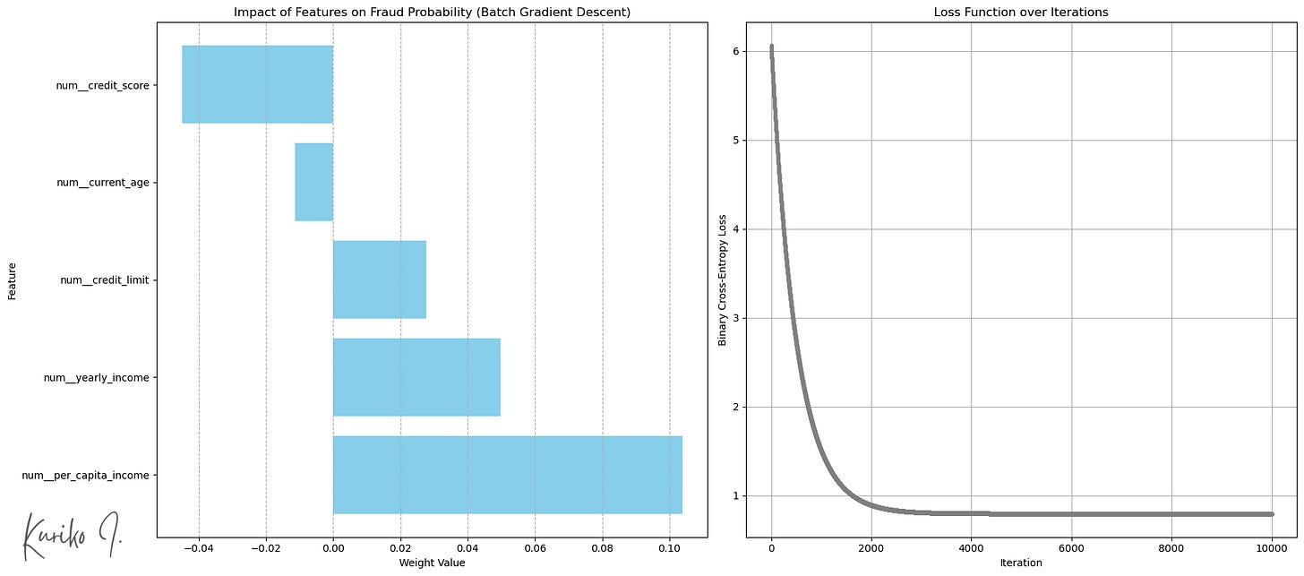

(Left: Weight by enter options (Backside: extra transaction), Proper: Price perform (learning_rate=0.001, i=10,000, m=50,000, n=5))

Imply Squared Error (MSE): 1.5752
R-squared: 0.0206
Imply Absolute Error (MAE): 1.0472

Time complexity: Coaching: O(n²m+n³) + Prediction: O(n)
House complexity: O(nm)
(m: coaching instance dimension, n: enter function dimension, assuming m >>> n)

Stochastic Gradient Descent

Batch GD makes use of your entire coaching dataset to compute gradient in every iteration step (epoch), which is computationally costly particularly when now we have tens of millions of dataset.

Stochastic Gradient Descent (SGD) alternatively,

1. usually shuffles the coaching knowledge initially of every epoch,
2. randomly choose a single coaching instance in every iteration,
3. calculates the gradient utilizing the instance, and
4. updates the mannequin’s weights and bias after processing every particular person coaching instance.

This leads to many weight updates per epoch (equal to the variety of coaching samples), many fast and computationally low-cost updates primarily based on particular person knowledge factors, permitting it to iterate by way of massive datasets a lot quicker.

Simulation

Much like Batch GD, we’ll outline the SGD class and run the prediction:

class StochasticGradientDescentLinearRegressor:
    def __init__(self, learning_rate=0.01, n_iterations=100, l2_penalty=0.01, random_state=None):
        self.learning_rate = learning_rate
        self.n_iterations = n_iterations
        self.l2_penalty = l2_penalty
        self.random_state = random_state
        self._rng = np.random.default_rng(seed=random_state)
        self.weights_history = []
        self.bias_history = []
        self.loss_history = []
        self.weights = None
        self.bias = None

    def _mse_loss_single(self, y_true, y_pred):
        return 0.5 * (y_pred - y_true)**2

    def match(self, X, y):
        n_samples, n_features = X.form
        self.weights = self._rng.random(n_features)
        self.bias = 0.0

        for epoch in vary(self.n_iterations):
            permutation = self._rng.permutation(n_samples)
            X_shuffled = X[permutation]
            y_shuffled = y[permutation]

            epoch_loss = 0
            for i in vary(n_samples):
                xi = X_shuffled[i]
                yi = y_shuffled[i]

                y_pred = np.dot(xi, self.weights) + self.bias
                dw = xi * (y_pred - yi) + self.l2_penalty * self.weights
                db = y_pred - yi

                self.weights -= self.learning_rate * dw
                self.bias -= self.learning_rate * db
                epoch_loss += self._mse_loss_single(yi, y_pred)

                if n_features >= 2:
                    self.weights_history.append(self.weights[:2].copy())
                elif n_features == 1:
                    self.weights_history.append(np.array([self.weights[0], 0]))
                self.bias_history.append(self.bias)
                self.loss_history.append(self._mse_loss_single(yi, y_pred) + (self.l2_penalty / (2 * n_samples)) * (np.sum(self.weights**2) + self.bias**2)) # Approx L2

            print(f"Epoch {epoch+1}/{self.n_iterations}, Loss: {epoch_loss/n_samples:.4f}")

    def predict(self, X):
        return np.dot(X, self.weights) + self.bias

mannequin = StochasticGradientDescentLinearRegressor(learning_rate=0.001, n_iterations=200, random_state=42)
mannequin.match(X=X_train_processed, y=y_train.values)
y_pred = mannequin.predict(X_test_processed)

Output:

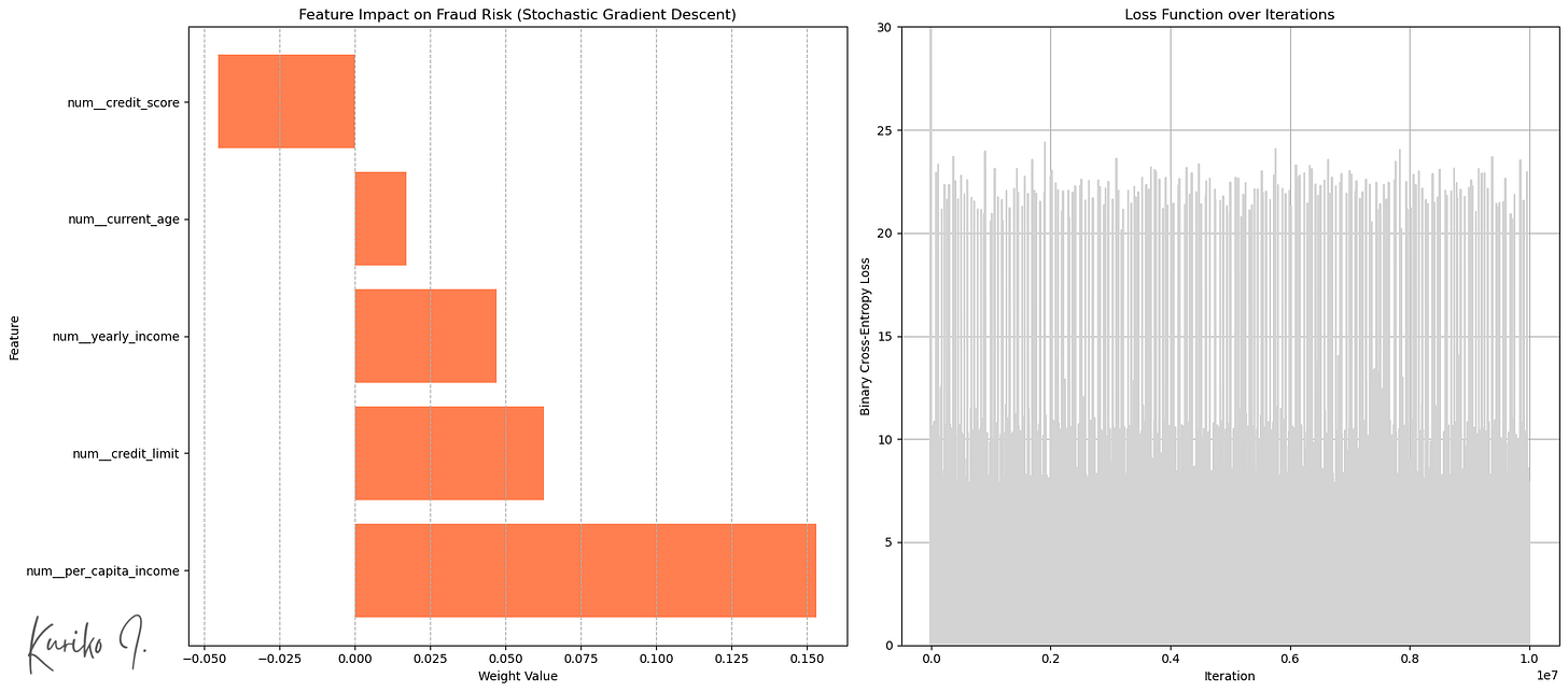
Left: Weight by enter options, Proper: Price perform (learning_rate=0.001, i=200, m=50,000, n=5)

SGD launched randomness into the optimization course of (fig. proper).

This “noise” may help the algorithm soar out of shallow native minima or saddle factors and doubtlessly discover higher areas of the parameter house.

Outcomes:
Imply Squared Error (MSE): 1.5808
R-squared: 0.0172
Imply Absolute Error (MAE): 1.0475

Time complexity: Coaching: O(n²m+n³) + Prediction: O(n)
House complexity: O(n) < BGD: O(nm)
(m: coaching instance dimension, n: enter function dimension, assuming m >>> n)

Conclusion

Whereas the easy linear mannequin is computationally environment friendly, its inherent simplicity usually prevents it from capturing complicated relationships throughout the knowledge.

Contemplating the trade-offs of varied modeling approaches towards particular aims is important for reaching optimum outcomes.

Reference

All photos, except in any other case famous, are by the writer.

The article makes use of artificial knowledge, licensed below Apache 2.0 for business use.

Creator: Kuriko IWAI

Portfolio / LinkedIn / Github